poco exposes a single method argument to
switch between density approximations. This vignette compares the
available backends on a small synthetic posterior so you can pick the
right trade-off for your problem.
Available methods
compression_methods()
#> [1] "mclust"     "mvdens_gmm" "mvdens_kde"
method |
Backend | Notes |
|---|---|---|
"mclust" |
mclust::Mclust() |
parametric GMM, BIC-based selection, fast & compact |
"mvdens_gmm" |
mvdens::fit.gmm() |
EM-based GMM, requires the suggested mvdens
package |
"mvdens_kde" |
mvdens::fit.kde() |
kernel density estimate, larger but non-parametric |
A toy posterior with correlated parameters
set.seed(1)
n_per <- 2000
draws <- rbind(
  mvtnorm::rmvnorm(
    n_per,
    mean = c(5.5, 2.0, 2.0),
    sigma = matrix(c(
      1.0, -0.14, 0.00,
      -0.14, 0.03, 0.00,
      0.00, 0.00, 0.05
    ), 3, 3, byrow = TRUE)
  ),
  mvtnorm::rmvnorm(
    n_per,
    mean = c(7.0, 1.8, 1.9),
    sigma = matrix(c(
      1.2, -0.18, 0.00,
      -0.18, 0.04, 0.00,
      0.00, 0.00, 0.06
    ), 3, 3, byrow = TRUE)
  )
)
colnames(draws) <- c("alpha", "beta", "sigma")
Compress with each method
mvdens_* methods require the suggested
mvdens package; we skip them gracefully when it is not
installed.
methods_to_try <- c("mclust")
if (requireNamespace("mvdens", quietly = TRUE)) {
  methods_to_try <- c(methods_to_try, "mvdens_gmm", "mvdens_kde")
}

fits <- lapply(methods_to_try, function(m) {
  compress_posterior(draws, method = m, n_components = 2)
})
#> ℹ mclust: trying all 14 covariance models c(EII, VII, EEI, VEI, EVI, VVI, EEE, VEE, EVE, VVE, EEV, VEV, EVV, VVV) and picking the best by BIC (n = 4000, d = 3).
#> ℹ mclust: selected model 'EEE' with G = 2 (BIC = -7,020.8) out of 14 candidate models: EII, VII, EEI, VEI, EVI, VVI, EEE, VEE, EVE, VVE, EEV, VEV, EVV, VVV.
#> Warning in .fit.gmm.internal(x, K, truncated = F, bounds = NA, min_cov = NULL,
#> : Solution not converged in1000, returning optimal found solution
names(fits) <- methods_to_try
Storage efficiency
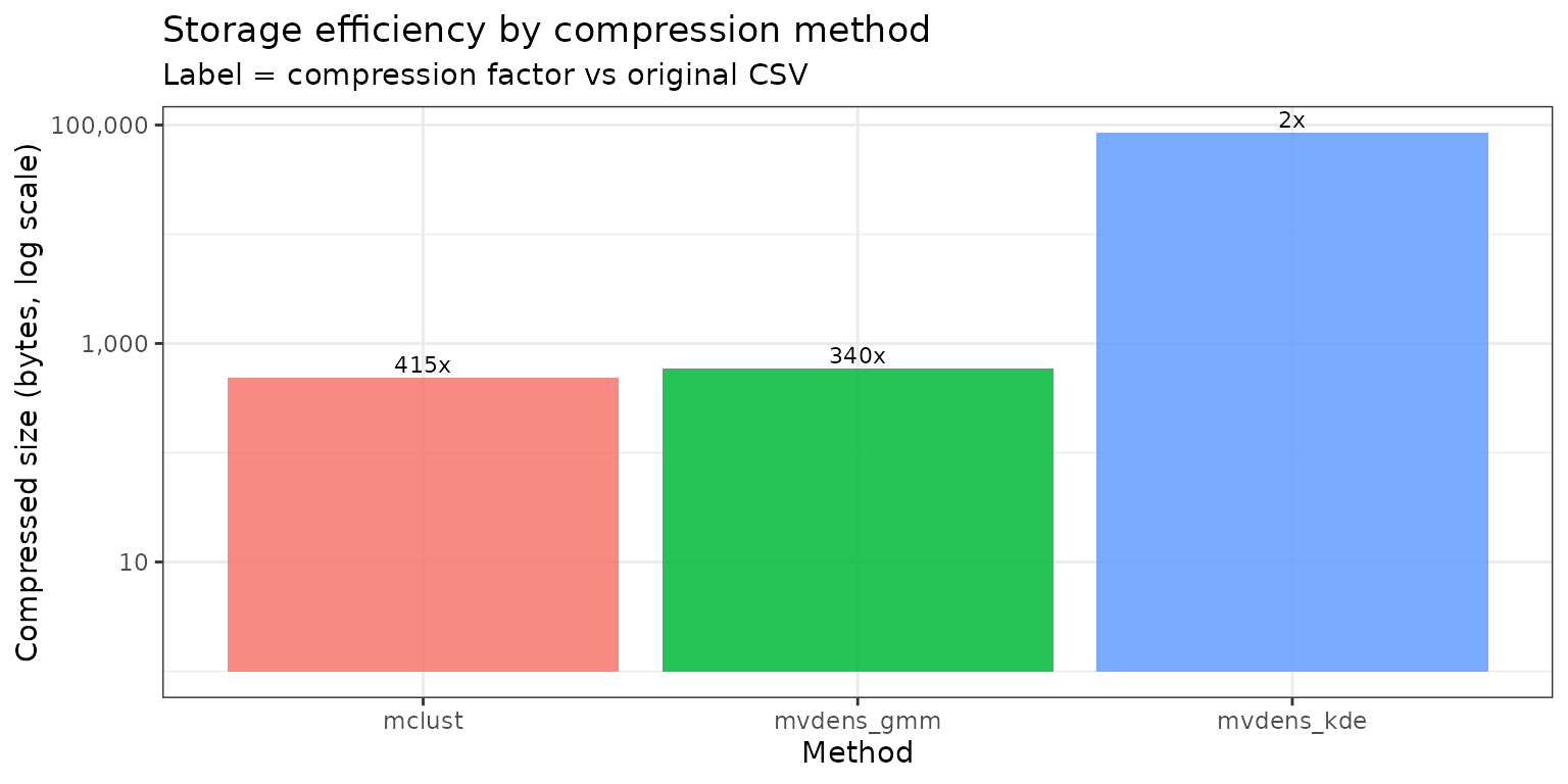
Compare compressed file sizes against the original posterior draws. Expected pattern: GMM-based methods are usually much smaller than KDE because they store only mixture parameters rather than all data points.
has_ggplot <- requireNamespace("ggplot2", quietly = TRUE)

tmp_dir <- tempfile("storage-benchmark-")
dir.create(tmp_dir, recursive = TRUE, showWarnings = FALSE)

csv_files <- file.path(tmp_dir, "posterior_draws.csv")
utils::write.csv(draws, csv_files, row.names = FALSE)

rds_paths <- file.path(tmp_dir, paste0("posterior_", names(fits), ".rds"))
for (i in seq_along(fits)) {
  saveRDS(fits[[i]], rds_paths[[i]], compress = "xz")
}

original_size <- as.numeric(file.size(csv_files))
compressed_sizes <- file.size(rds_paths)
compression_x <- original_size / compressed_sizes
pct_of_original <- 100 * compressed_sizes / original_size

for (i in seq_along(compressed_sizes)) {
  cat(
    sprintf(
      "%-12s %10s bytes (%.2f%% of original, %.0fx compression)\n",
      paste0(names(fits)[[i]], ":"),
      format(compressed_sizes[[i]], big.mark = ","),
      pct_of_original[[i]],
      compression_x[[i]]
    )
  )
}
#> mclust:             488 bytes (0.24% of original, 415x compression)
#> mvdens_gmm:         596 bytes (0.29% of original, 340x compression)
#> mvdens_kde:      84,660 bytes (41.76% of original, 2x compression)

storage_df <- data.frame(
  method = names(fits),
  bytes = as.numeric(compressed_sizes),
  pct_of_original = as.numeric(pct_of_original),
  compression_x = as.numeric(compression_x)
)
storage_df <- storage_df[order(storage_df$bytes), ]
print(storage_df)
#>       method bytes pct_of_original compression_x
#> 1     mclust   488       0.2407356    415.393443
#> 2 mvdens_gmm   596       0.2940132    340.120805
#> 3 mvdens_kde 84660      41.7636844      2.394425

if (has_ggplot) {
  ggplot2::ggplot(
    storage_df,
    ggplot2::aes(x = reorder(method, bytes), y = bytes, fill = method)
  ) +
    ggplot2::geom_col(alpha = 0.85) +
    ggplot2::geom_text(
      ggplot2::aes(label = sprintf("%.0fx", compression_x)),
      vjust = -0.3,
      size = 3
    ) +
    ggplot2::scale_y_log10(labels = scales::label_number(big.mark = ",")) +
    ggplot2::labs(
      title = "Storage efficiency by compression method",
      subtitle = "Label = compression factor vs original CSV",
      x = "Method",
      y = "Compressed size (bytes, log scale)"
    ) +
    ggplot2::theme_bw() +
    ggplot2::theme(legend.position = "none")
} else {
  message("Install suggested package 'ggplot2' to render the storage efficiency plot.")
}
Sample regeneration
All methods support [sample_posterior()] with the same interface:
regen <- lapply(fits, sample_posterior, n_draws = 2000)

sapply(regen, function(s) {
  c(mean_alpha = mean(s[, "alpha"]),
    mean_beta  = mean(s[, "beta"]),
    mean_sigma = mean(s[, "sigma"]),
    cor_alpha_beta = cor(s[, "alpha"], s[, "beta"]))
})
#>                    mclust mvdens_gmm mvdens_kde
#> mean_alpha      6.2821786  6.2789029  6.2872840
#> mean_beta       1.8942849  1.8938995  1.8896709
#> mean_sigma      1.9418046  1.9412992  1.9322318
#> cor_alpha_beta -0.8738303 -0.8500717 -0.8615243
Pairwise comparison plot
Visual overlap between original draws (gray) and regenerated samples.
if (requireNamespace("ggplot2", quietly = TRUE) &&
    requireNamespace("patchwork", quietly = TRUE)) {
  draws_df <- as.data.frame(draws)
  palette_map <- c(mvdens_gmm = "red", mvdens_kde = "darkgreen", mclust = "blue")
  has_ggside <- requireNamespace("ggside", quietly = TRUE)

  plot_pairwise <- function(var1, var2) {
    p <- ggplot2::ggplot(mapping = ggplot2::aes_string(x = var1, y = var2)) +
      ggplot2::geom_point(
        data = draws_df,
        alpha = 0.15,
        size = 0.5,
        color = "gray50"
      ) +
      ggplot2::labs(
        x = var1,
        y = var2,
        title = paste(var1, "vs", var2)
      ) +
      ggplot2::theme_bw() +
      ggplot2::theme(plot.title = ggplot2::element_text(size = 9))

    if (has_ggside) {
      p <- p +
        ggside::geom_xsidedensity(
          data = draws_df,
          ggplot2::aes(y = ..density..),
          color = "gray50",
          alpha = 0.8
        ) +
        ggside::geom_ysidedensity(
          data = draws_df,
          ggplot2::aes(x = ..density..),
          color = "gray50",
          alpha = 0.8
        ) +
        ggside::theme_ggside_void()
    }

    for (method_name in names(regen)) {
      regen_df <- as.data.frame(regen[[method_name]])
      p <- p + ggplot2::geom_point(
        data = regen_df,
        alpha = 0.4,
        size = 0.5,
        color = unname(palette_map[method_name])
      )

      if (has_ggside) {
        p <- p +
          ggside::geom_xsidedensity(
            data = regen_df,
            ggplot2::aes(y = ..density..),
            color = unname(palette_map[method_name]),
            alpha = 0.8
          ) +
          ggside::geom_ysidedensity(
            data = regen_df,
            ggplot2::aes(x = ..density..),
            color = unname(palette_map[method_name]),
            alpha = 0.8
          )
      }
    }
    p
  }

  param_names <- colnames(draws_df)
  plot_list <- list()
  idx <- 1
  for (i in 1:(length(param_names) - 1)) {
    for (j in (i + 1):length(param_names)) {
      plot_list[[idx]] <- plot_pairwise(param_names[i], param_names[j])
      idx <- idx + 1
    }
  }

  ncol_grid <- ceiling(sqrt(length(plot_list)))
  combined_plot <- patchwork::wrap_plots(plot_list, ncol = ncol_grid) +
    patchwork::plot_annotation(
      title = "Original (gray) | mvdens GMM (red) | mvdens KDE (green) | mclust GMM (blue)"
    )

  combined_plot
} else {
  message("Install suggested packages 'ggplot2' and 'patchwork' to render combined_plot.")
}
#> Warning: `aes_string()` was deprecated in ggplot2 3.0.0.
#> ℹ Please use tidy evaluation idioms with `aes()`.
#> ℹ See also `vignette("ggplot2-in-packages")` for more information.
#> This warning is displayed once per session.
#> Call `lifecycle::last_lifecycle_warnings()` to see where this warning was
#> generated.
#> Warning: The dot-dot notation (`..density..`) was deprecated in ggplot2 3.4.0.
#> ℹ Please use `after_stat(density)` instead.
#> This warning is displayed once per session.
#> Call `lifecycle::last_lifecycle_warnings()` to see where this warning was
#> generated.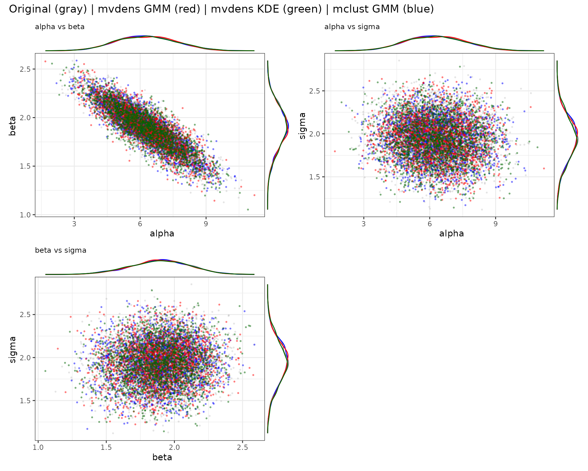
Compression runtime benchmark
Benchmark compression on the same synthetic posterior matrix for each backend and visualize runtime.
if (requireNamespace("microbenchmark", quietly = TRUE) &&
    requireNamespace("ggplot2", quietly = TRUE)) {
  benchmark_draws <- draws
  has_mvdens <- requireNamespace("mvdens", quietly = TRUE)

  bench_parts <- list(
    mclust_gmm = microbenchmark::microbenchmark(
      mclust_gmm = compress_posterior(
        benchmark_draws,
        method = "mclust",
        n_components = 2
      ),
      times = 10,
      unit = "ms"
    )
  )

  if (has_mvdens) {
    bench_parts$mvdens_gmm <- microbenchmark::microbenchmark(
      mvdens_gmm = compress_posterior(
        benchmark_draws,
        method = "mvdens_gmm",
        n_components = 2
      ),
      times = 10,
      unit = "ms"
    )

    bench_parts$mvdens_kde <- microbenchmark::microbenchmark(
      mvdens_kde = compress_posterior(
        benchmark_draws,
        method = "mvdens_kde"
      ),
      times = 10,
      unit = "ms"
    )
  }

  bench_compression <- do.call(
    rbind,
    lapply(bench_parts, function(x) {
      out <- as.data.frame(x)
      out$time_ms <- out$time / 1e6
      out
    })
  )

  print(bench_compression[, c("expr", "time_ms")])

  ggplot2::ggplot(bench_compression, ggplot2::aes(x = expr, y = time_ms, color = expr)) +
    ggplot2::geom_boxplot(outlier.shape = NA, alpha = 0.2) +
    ggplot2::geom_jitter(width = 0.12, alpha = 0.7, size = 2) +
    ggplot2::labs(
      title = "Compression runtime by method",
      x = "Method",
      y = "Time (ms)"
    ) +
    ggplot2::theme_bw() +
    ggplot2::theme(legend.position = "none")
} else {
  message("Install suggested packages 'microbenchmark' and 'ggplot2' to run this benchmark.")
}
#> ℹ mclust: trying all 14 covariance models c(EII, VII, EEI, VEI, EVI, VVI, EEE, VEE, EVE, VVE, EEV, VEV, EVV, VVV) and picking the best by BIC (n = 4000, d = 3).
#> ℹ mclust: selected model 'EEE' with G = 2 (BIC = -7,021.44) out of 14 candidate models: EII, VII, EEI, VEI, EVI, VVI, EEE, VEE, EVE, VVE, EEV, VEV, EVV, VVV.
#> ℹ mclust: trying all 14 covariance models c(EII, VII, EEI, VEI, EVI, VVI, EEE, VEE, EVE, VVE, EEV, VEV, EVV, VVV) and picking the best by BIC (n = 4000, d = 3).
#> ℹ mclust: selected model 'EEE' with G = 2 (BIC = -7,025.4) out of 14 candidate models: EII, VII, EEI, VEI, EVI, VVI, EEE, VEE, EVE, VVE, EEV, VEV, EVV, VVV.
#> ℹ mclust: trying all 14 covariance models c(EII, VII, EEI, VEI, EVI, VVI, EEE, VEE, EVE, VVE, EEV, VEV, EVV, VVV) and picking the best by BIC (n = 4000, d = 3).
#> ℹ mclust: selected model 'EEE' with G = 2 (BIC = -7,024.56) out of 14 candidate models: EII, VII, EEI, VEI, EVI, VVI, EEE, VEE, EVE, VVE, EEV, VEV, EVV, VVV.
#> ℹ mclust: trying all 14 covariance models c(EII, VII, EEI, VEI, EVI, VVI, EEE, VEE, EVE, VVE, EEV, VEV, EVV, VVV) and picking the best by BIC (n = 4000, d = 3).
#> ℹ mclust: selected model 'EEE' with G = 2 (BIC = -7,021.4) out of 14 candidate models: EII, VII, EEI, VEI, EVI, VVI, EEE, VEE, EVE, VVE, EEV, VEV, EVV, VVV.
#> ℹ mclust: trying all 14 covariance models c(EII, VII, EEI, VEI, EVI, VVI, EEE, VEE, EVE, VVE, EEV, VEV, EVV, VVV) and picking the best by BIC (n = 4000, d = 3).
#> ℹ mclust: selected model 'EEE' with G = 2 (BIC = -7,024.78) out of 14 candidate models: EII, VII, EEI, VEI, EVI, VVI, EEE, VEE, EVE, VVE, EEV, VEV, EVV, VVV.
#> ℹ mclust: trying all 14 covariance models c(EII, VII, EEI, VEI, EVI, VVI, EEE, VEE, EVE, VVE, EEV, VEV, EVV, VVV) and picking the best by BIC (n = 4000, d = 3).
#> ℹ mclust: selected model 'VEE' with G = 2 (BIC = -7,024.56) out of 14 candidate models: EII, VII, EEI, VEI, EVI, VVI, EEE, VEE, EVE, VVE, EEV, VEV, EVV, VVV.
#> ℹ mclust: trying all 14 covariance models c(EII, VII, EEI, VEI, EVI, VVI, EEE, VEE, EVE, VVE, EEV, VEV, EVV, VVV) and picking the best by BIC (n = 4000, d = 3).
#> ℹ mclust: selected model 'EEE' with G = 2 (BIC = -7,021.48) out of 14 candidate models: EII, VII, EEI, VEI, EVI, VVI, EEE, VEE, EVE, VVE, EEV, VEV, EVV, VVV.
#> ℹ mclust: trying all 14 covariance models c(EII, VII, EEI, VEI, EVI, VVI, EEE, VEE, EVE, VVE, EEV, VEV, EVV, VVV) and picking the best by BIC (n = 4000, d = 3).
#> ℹ mclust: selected model 'EEE' with G = 2 (BIC = -7,023.14) out of 14 candidate models: EII, VII, EEI, VEI, EVI, VVI, EEE, VEE, EVE, VVE, EEV, VEV, EVV, VVV.
#> ℹ mclust: trying all 14 covariance models c(EII, VII, EEI, VEI, EVI, VVI, EEE, VEE, EVE, VVE, EEV, VEV, EVV, VVV) and picking the best by BIC (n = 4000, d = 3).
#> ℹ mclust: selected model 'EEE' with G = 2 (BIC = -7,024.86) out of 14 candidate models: EII, VII, EEI, VEI, EVI, VVI, EEE, VEE, EVE, VVE, EEV, VEV, EVV, VVV.
#> ℹ mclust: trying all 14 covariance models c(EII, VII, EEI, VEI, EVI, VVI, EEE, VEE, EVE, VVE, EEV, VEV, EVV, VVV) and picking the best by BIC (n = 4000, d = 3).
#> ℹ mclust: selected model 'EEE' with G = 2 (BIC = -7,020.93) out of 14 candidate models: EII, VII, EEI, VEI, EVI, VVI, EEE, VEE, EVE, VVE, EEV, VEV, EVV, VVV.
#> Warning in .fit.gmm.internal(x, K, truncated = F, bounds = NA, min_cov = NULL,
#> : Solution not converged in1000, returning optimal found solution
#> Warning in .fit.gmm.internal(x, K, truncated = F, bounds = NA, min_cov = NULL,
#> : Solution not converged in1000, returning optimal found solution
#> Warning in .fit.gmm.internal(x, K, truncated = F, bounds = NA, min_cov = NULL,
#> : Solution not converged in1000, returning optimal found solution
#> Warning in .fit.gmm.internal(x, K, truncated = F, bounds = NA, min_cov = NULL,
#> : Solution not converged in1000, returning optimal found solution
#> Warning in .fit.gmm.internal(x, K, truncated = F, bounds = NA, min_cov = NULL,
#> : Solution not converged in1000, returning optimal found solution
#>                     expr   time_ms
#> mclust_gmm.1  mclust_gmm  2286.856
#> mclust_gmm.2  mclust_gmm  3111.911
#> mclust_gmm.3  mclust_gmm  2354.723
#> mclust_gmm.4  mclust_gmm  2593.196
#> mclust_gmm.5  mclust_gmm  2988.332
#> mclust_gmm.6  mclust_gmm  2277.236
#> mclust_gmm.7  mclust_gmm  2205.143
#> mclust_gmm.8  mclust_gmm  2309.309
#> mclust_gmm.9  mclust_gmm  2461.917
#> mclust_gmm.10 mclust_gmm  2221.798
#> mvdens_gmm.1  mvdens_gmm  8884.433
#> mvdens_gmm.2  mvdens_gmm  8344.515
#> mvdens_gmm.3  mvdens_gmm  9439.323
#> mvdens_gmm.4  mvdens_gmm  7306.413
#> mvdens_gmm.5  mvdens_gmm 27692.659
#> mvdens_gmm.6  mvdens_gmm 27837.916
#> mvdens_gmm.7  mvdens_gmm 27831.938
#> mvdens_gmm.8  mvdens_gmm  6894.103
#> mvdens_gmm.9  mvdens_gmm 27266.869
#> mvdens_gmm.10 mvdens_gmm 27354.119
#> mvdens_kde.1  mvdens_kde  5319.903
#> mvdens_kde.2  mvdens_kde  4214.980
#> mvdens_kde.3  mvdens_kde  4557.528
#> mvdens_kde.4  mvdens_kde  4433.683
#> mvdens_kde.5  mvdens_kde  3922.493
#> mvdens_kde.6  mvdens_kde  3854.048
#> mvdens_kde.7  mvdens_kde  4373.774
#> mvdens_kde.8  mvdens_kde  4035.744
#> mvdens_kde.9  mvdens_kde  4039.596
#> mvdens_kde.10 mvdens_kde  4000.393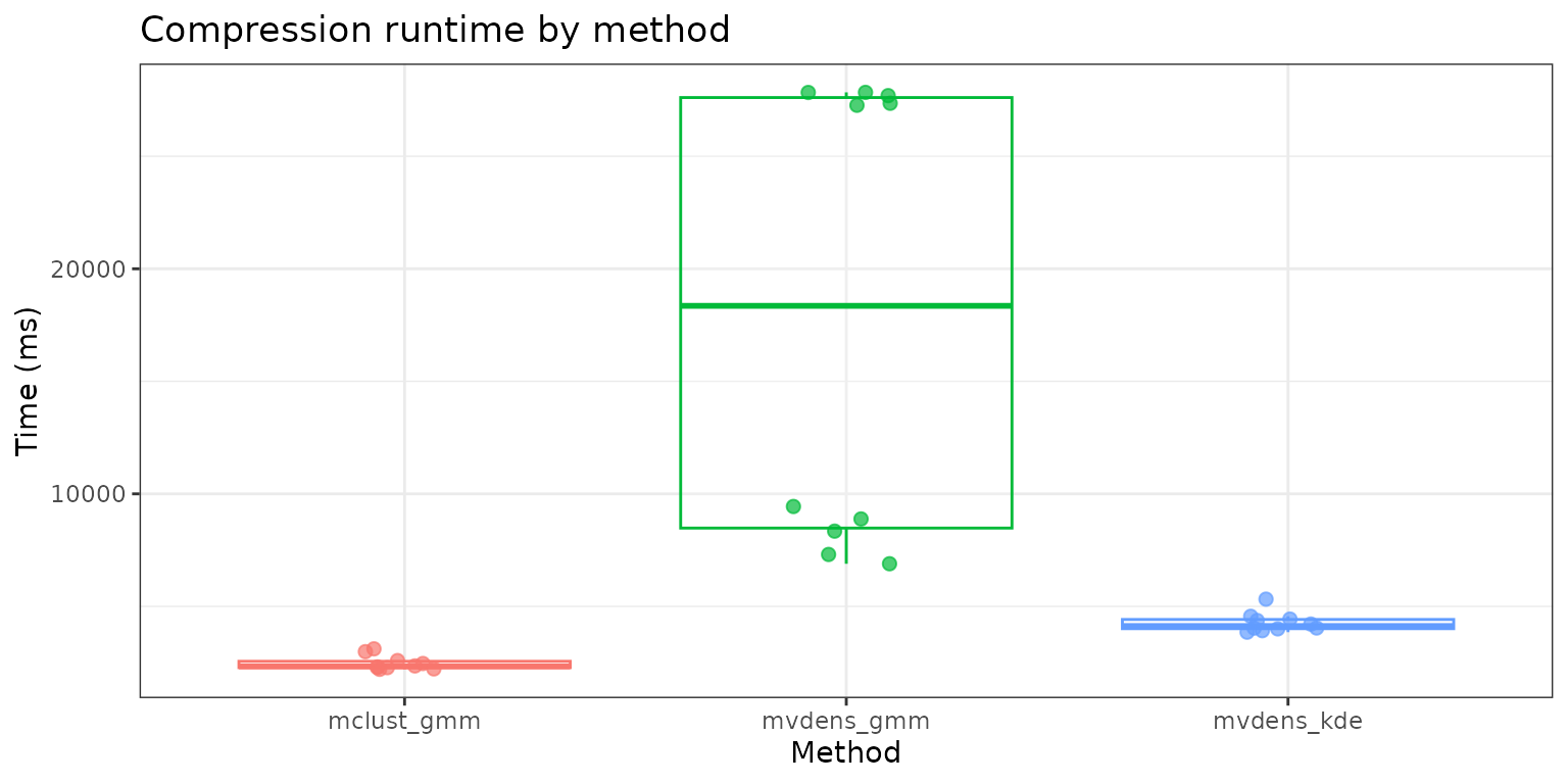
Picking a method
-
"mclust": fastest path; great default for parameter counts in the hundreds to low thousands. -
"mvdens_gmm": alternative EM-based GMM, useful for cross-checks. -
"mvdens_kde": non-parametric, larger storage footprint, useful when the posterior is far from a mixture of Gaussians.
Session info
sessionInfo()
#> R version 4.6.0 (2026-04-24)
#> Platform: x86_64-pc-linux-gnu
#> Running under: Ubuntu 24.04.4 LTS
#>
#> Matrix products: default
#> BLAS:   /usr/lib/x86_64-linux-gnu/openblas-pthread/libblas.so.3
#> LAPACK: /usr/lib/x86_64-linux-gnu/openblas-pthread/libopenblasp-r0.3.26.so;  LAPACK version 3.12.0
#>
#> locale:
#>  [1] LC_CTYPE=C.UTF-8       LC_NUMERIC=C           LC_TIME=C.UTF-8
#>  [4] LC_COLLATE=C.UTF-8     LC_MONETARY=C.UTF-8    LC_MESSAGES=C.UTF-8
#>  [7] LC_PAPER=C.UTF-8       LC_NAME=C              LC_ADDRESS=C
#> [10] LC_TELEPHONE=C         LC_MEASUREMENT=C.UTF-8 LC_IDENTIFICATION=C
#>
#> time zone: UTC
#> tzcode source: system (glibc)
#>
#> attached base packages:
#> [1] stats     graphics  grDevices utils     datasets  methods   base
#>
#> other attached packages:
#> [1] mvtnorm_1.3-7 poco_0.2.0
#>
#> loaded via a namespace (and not attached):
#>  [1] ks_1.15.1            sass_0.4.10          generics_0.1.4
#>  [4] KernSmooth_2.23-26   lattice_0.22-9       pracma_2.4.6
#>  [7] digest_0.6.39        magrittr_2.0.5       evaluate_1.0.5
#> [10] grid_4.6.0           RColorBrewer_1.1-3   instantiate_0.2.3
#> [13] fastmap_1.2.0        jsonlite_2.0.0       Matrix_1.7-5
#> [16] ggside_0.4.1         processx_3.9.0       mclust_6.1.2
#> [19] ps_1.9.3             scales_1.4.0         microbenchmark_1.5.0
#> [22] textshaping_1.0.5    jquerylib_0.1.4      cli_3.6.6
#> [25] rlang_1.2.0          withr_3.0.2          cachem_1.1.0
#> [28] yaml_2.3.12          otel_0.2.0           tools_4.6.0
#> [31] dplyr_1.2.1          ggplot2_4.0.3        mvdens_1.1.0
#> [34] vctrs_0.7.3          R6_2.6.1             lifecycle_1.0.5
#> [37] fs_2.1.0             htmlwidgets_1.6.4    ragg_1.5.2
#> [40] pkgconfig_2.0.3      desc_1.4.3           callr_3.7.6
#> [43] pkgdown_2.2.0        bslib_0.10.0         pillar_1.11.1
#> [46] gtable_0.3.6         glue_1.8.1           systemfonts_1.3.2
#> [49] xfun_0.57            tibble_3.3.1         tidyselect_1.2.1
#> [52] knitr_1.51           farver_2.1.2         patchwork_1.3.2
#> [55] htmltools_0.5.9      labeling_0.4.3       rmarkdown_2.31
#> [58] compiler_4.6.0       S7_0.2.2