Introduction to Tidy Transcriptomics
Maria Doyle, Peter MacCallum Cancer Centre1
Stefano Mangiola, Walter and Eliza Hall Institute2
Source:vignettes/tidytranscriptomics.Rmd
tidytranscriptomics.RmdBackground
Background information and setup instructions for this workshop can be found here.
Part 1 Bulk RNA-seq with tidybulk
This workshop will present how to perform analysis of RNA sequencing data following the tidy data paradigm (Wickham and others 2014). The tidy data paradigm provides a standard way to organise data values within a dataset, where each variable is a column, each observation is a row, and data is manipulated using an easy-to-understand vocabulary. Most importantly, the data structure remains consistent across manipulation and analysis functions.
This can be achieved for RNA sequencing data with the tidybulk, tidyHeatmap (Mangiola and Papenfuss 2020) and tidyverse (Wickham et al. 2019) packages. The tidybulk package provides a tidy data structure and a modular framework for bulk transcriptional analyses. tidyHeatmap provides a tidy implementation of ComplexHeatmap. These packages are part of the tidytranscriptomics suite that introduces a tidy approach to RNA sequencing data representation and analysis
Acknowledgements
Some of the material in Part 1 was adapted from an R for RNA sequencing workshop first run here. Use of the airway dataset was inspired by the DESeq2 vignette.
![]()
Introduction
Measuring gene expression on a genome-wide scale has become common practice over the last two decades or so, with microarrays predominantly used pre-2008. With the advent of next generation sequencing technology in 2008, an increasing number of scientists use this technology to measure and understand changes in gene expression in often complex systems. As sequencing costs have decreased, using RNA sequencing to simultaneously measure the expression of tens of thousands of genes for multiple samples has never been easier. The cost of these experiments has now moved from generating the data to storing and analysing it.
There are many steps involved in analysing an RNA sequencing dataset. Sequenced reads are aligned to a reference genome, then the number of reads mapped to each gene can be counted. This results in a table of counts, which is what we perform statistical analyses on in R. While mapping and counting are important and necessary tasks, today we will be starting from the count data and showing how differential expression analysis can be performed in a friendly way using the Bioconductor package, tidybulk.
First, let’s load all the packages we will need to analyse the data.
Note: you should load the tidybulk library after the tidyverse core packages for best integration.
# load libraries

# dataset
library(airway)

# tidyverse core packages
library(tibble)
library(dplyr)
library(tidyr)
library(readr)
library(stringr)
library(ggplot2)

# tidyverse-friendly packages
library(plotly)
library(ggrepel)
library(GGally)
library(tidyHeatmap)
library(tidybulk)
Plot settings. Set the colours and theme we will use for our plots.
# Use colourblind-friendly colours
friendly_cols <- dittoSeq::dittoColors()

# Set theme
custom_theme <-
  list(
    scale_fill_manual(values = friendly_cols),
    scale_color_manual(values = friendly_cols),
    theme_bw() +
      theme(
        panel.border = element_blank(),
        axis.line = element_line(),
        panel.grid.major = element_line(size = 0.2),
        panel.grid.minor = element_line(size = 0.1),
        text = element_text(size = 12),
        legend.position = "bottom",
        strip.background = element_blank(),
        axis.title.x = element_text(margin = margin(t = 10, r = 10, b = 10, l = 10)),
        axis.title.y = element_text(margin = margin(t = 10, r = 10, b = 10, l = 10)),
        axis.text.x = element_text(angle = 30, hjust = 1, vjust = 1)
      )
  )
Setting up the data
Here we will perform our analysis using the data from the airway package. The airway data comes from the paper by (Himes et al. 2014); and it includes 8 samples from human airway smooth muscle cells, from 4 cell lines. For each cell line treated (with dexamethasone) and untreated (negative control) a sample has undergone RNA sequencing and gene counts have been generated.
The airway data is stored as a Bioconductor RangedSummarizedExperiment object. We will convert this object into a tidybulk tibble. A tibble is the tidyverse table format.
In this workshop we will be using the tidyverse pipe %>%. This ‘pipes’ the output from the command on the left into the command on the right/below. Using the pipe is not essential but it reduces the amount of code we need to write when we have multiple steps (as we’ll see later). It also can make the steps clearer and easier to see. For more details on the pipe see here.
# load airway RNA sequencing data
data(airway)

# convert to tidybulk tibble
counts_airway <-
  airway %>%
  tidybulk()

# take a look
counts_airway
#> # A tibble: 512,816 x 12
#>    feature sample counts SampleName cell  dex   albut Run   avgLength Experiment
#>    <fct>   <fct>   <int> <fct>      <fct> <fct> <fct> <fct>     <int> <fct>
#>  1 ENSG00… SRR10…    679 GSM1275862 N613… untrt untrt SRR1…       126 SRX384345
#>  2 ENSG00… SRR10…      0 GSM1275862 N613… untrt untrt SRR1…       126 SRX384345
#>  3 ENSG00… SRR10…    467 GSM1275862 N613… untrt untrt SRR1…       126 SRX384345
#>  4 ENSG00… SRR10…    260 GSM1275862 N613… untrt untrt SRR1…       126 SRX384345
#>  5 ENSG00… SRR10…     60 GSM1275862 N613… untrt untrt SRR1…       126 SRX384345
#>  6 ENSG00… SRR10…      0 GSM1275862 N613… untrt untrt SRR1…       126 SRX384345
#>  7 ENSG00… SRR10…   3251 GSM1275862 N613… untrt untrt SRR1…       126 SRX384345
#>  8 ENSG00… SRR10…   1433 GSM1275862 N613… untrt untrt SRR1…       126 SRX384345
#>  9 ENSG00… SRR10…    519 GSM1275862 N613… untrt untrt SRR1…       126 SRX384345
#> 10 ENSG00… SRR10…    394 GSM1275862 N613… untrt untrt SRR1…       126 SRX384345
#> # … with 512,806 more rows, and 2 more variables: Sample <fct>, BioSample <fct>
The counts_airway object contains information about genes and samples, the first column has the Ensembl gene identifier, the second column has the sample identifier and the third column has the gene transcription abundance. The abundance is the number of reads aligning to the gene in each experimental sample. The remaining columns include sample-wise information. The dex column tells us whether the samples are treated or untreated and the cell column tells us what cell line they are from. We can shorten the sample names. We can remove the SRR1039 prefix that’s present in all of them, as shorter names can fit better in some of the plots we will create. We can use mutate() together with str_replace() to remove the SRR1039 string from the sample column. We can get the gene symbols for these Ensembl gene ids using the Bioconductor annotation package for human, org.Hs.eg.db and add them as a column using mutate again. With tidyverse, all above steps can be linked with the %>%, as shown below. This has the benefits that * no temporary variables need to be created * less typing is required * the steps can be seen more clearly.
# setup data workflow
counts_tt <-
  airway %>%
  tidybulk() %>%
  mutate(sample = str_remove(sample, "SRR1039")) %>%
  mutate(symbol = AnnotationDbi::mapIds(org.Hs.eg.db::org.Hs.eg.db,
    keys = as.character(feature),
    keytype = "ENSEMBL",
    column = "SYMBOL",
    multiVals = "first"
  ))
#>
#> 'select()' returned 1:many mapping between keys and columns
# take a look
counts_tt
#> # A tibble: 512,816 x 13
#>    feature sample counts SampleName cell  dex   albut Run   avgLength Experiment
#>    <fct>   <chr>   <int> <fct>      <fct> <fct> <fct> <fct>     <int> <fct>
#>  1 ENSG00… 508       679 GSM1275862 N613… untrt untrt SRR1…       126 SRX384345
#>  2 ENSG00… 508         0 GSM1275862 N613… untrt untrt SRR1…       126 SRX384345
#>  3 ENSG00… 508       467 GSM1275862 N613… untrt untrt SRR1…       126 SRX384345
#>  4 ENSG00… 508       260 GSM1275862 N613… untrt untrt SRR1…       126 SRX384345
#>  5 ENSG00… 508        60 GSM1275862 N613… untrt untrt SRR1…       126 SRX384345
#>  6 ENSG00… 508         0 GSM1275862 N613… untrt untrt SRR1…       126 SRX384345
#>  7 ENSG00… 508      3251 GSM1275862 N613… untrt untrt SRR1…       126 SRX384345
#>  8 ENSG00… 508      1433 GSM1275862 N613… untrt untrt SRR1…       126 SRX384345
#>  9 ENSG00… 508       519 GSM1275862 N613… untrt untrt SRR1…       126 SRX384345
#> 10 ENSG00… 508       394 GSM1275862 N613… untrt untrt SRR1…       126 SRX384345
#> # … with 512,806 more rows, and 3 more variables: Sample <fct>,
#> #   BioSample <fct>, symbol <chr>
From this tidybulk tibble, we can perform differential expression analysis with the tidybulk package.
Filtering lowly transcribed genes
Genes with very low counts across all libraries provide little evidence for differential expression and they can interfere with some of the statistical approximations that are used later in the pipeline. They also add to the multiple testing burden when estimating false discovery rates, reducing power to detect differentially expressed genes. These genes should be filtered out prior to further analysis.
We can perform the filtering using tidybulk keep_abundant or identify_abundant. These functions can use the edgeR filterByExpr function described in (Law et al. 2016) to automatically identify the genes with adequate abundance for differential expression testing. By default, this will keep genes with ~10 counts in a minimum number of samples, the number of the samples in the smallest group. In this dataset the smallest group size is four (as we have four dex-treated samples versus four untreated). Alternatively, we could use identify_abundant to identify which genes are abundant or not (TRUE/FALSE), rather than just keeping the abundant ones.
# Filtering counts
counts_filtered <- counts_tt %>% keep_abundant(factor_of_interest = dex)

# take a look
counts_filtered
#> # A tibble: 127,408 x 14
#>    feature sample counts SampleName cell  dex   albut Run   avgLength Experiment
#>    <fct>   <chr>   <int> <fct>      <fct> <fct> <fct> <fct>     <int> <fct>
#>  1 ENSG00… 508       679 GSM1275862 N613… untrt untrt SRR1…       126 SRX384345
#>  2 ENSG00… 508       467 GSM1275862 N613… untrt untrt SRR1…       126 SRX384345
#>  3 ENSG00… 508       260 GSM1275862 N613… untrt untrt SRR1…       126 SRX384345
#>  4 ENSG00… 508        60 GSM1275862 N613… untrt untrt SRR1…       126 SRX384345
#>  5 ENSG00… 508      3251 GSM1275862 N613… untrt untrt SRR1…       126 SRX384345
#>  6 ENSG00… 508      1433 GSM1275862 N613… untrt untrt SRR1…       126 SRX384345
#>  7 ENSG00… 508       519 GSM1275862 N613… untrt untrt SRR1…       126 SRX384345
#>  8 ENSG00… 508       394 GSM1275862 N613… untrt untrt SRR1…       126 SRX384345
#>  9 ENSG00… 508       172 GSM1275862 N613… untrt untrt SRR1…       126 SRX384345
#> 10 ENSG00… 508      2112 GSM1275862 N613… untrt untrt SRR1…       126 SRX384345
#> # … with 127,398 more rows, and 4 more variables: Sample <fct>,
#> #   BioSample <fct>, symbol <chr>, .abundant <lgl>
After running keep_abundant we have a column called .abundant containing TRUE (identify_abundant would have TRUE/FALSE).
Scaling counts to normalise
Scaling of counts, normalisation, is performed to eliminate uninteresting differences between samples due to sequencing depth or composition. A more detailed explanation can be found here. In the tidybulk package the function scale_abundance generates scaled counts, with scaling factors calculated on abundant (filtered) transcripts and applied to all transcripts. We can choose from different normalisation methods. Here we will use the default, edgeR’s trimmed mean of M values (TMM), (Robinson and Oshlack 2010). TMM normalisation (and most scaling normalisation methods) scale relative to one sample.
# Scaling counts
counts_scaled <- counts_filtered %>% scale_abundance()

# take a look
counts_scaled
#> # A tibble: 127,408 x 17
#>    feature sample counts SampleName cell  dex   albut Run   avgLength Experiment
#>    <fct>   <chr>   <int> <fct>      <fct> <fct> <fct> <fct>     <int> <fct>
#>  1 ENSG00… 508       679 GSM1275862 N613… untrt untrt SRR1…       126 SRX384345
#>  2 ENSG00… 508       467 GSM1275862 N613… untrt untrt SRR1…       126 SRX384345
#>  3 ENSG00… 508       260 GSM1275862 N613… untrt untrt SRR1…       126 SRX384345
#>  4 ENSG00… 508        60 GSM1275862 N613… untrt untrt SRR1…       126 SRX384345
#>  5 ENSG00… 508      3251 GSM1275862 N613… untrt untrt SRR1…       126 SRX384345
#>  6 ENSG00… 508      1433 GSM1275862 N613… untrt untrt SRR1…       126 SRX384345
#>  7 ENSG00… 508       519 GSM1275862 N613… untrt untrt SRR1…       126 SRX384345
#>  8 ENSG00… 508       394 GSM1275862 N613… untrt untrt SRR1…       126 SRX384345
#>  9 ENSG00… 508       172 GSM1275862 N613… untrt untrt SRR1…       126 SRX384345
#> 10 ENSG00… 508      2112 GSM1275862 N613… untrt untrt SRR1…       126 SRX384345
#> # … with 127,398 more rows, and 7 more variables: Sample <fct>,
#> #   BioSample <fct>, symbol <chr>, .abundant <lgl>, TMM <dbl>,
#> #   multiplier <dbl>, counts_scaled <dbl>
After we run scale_abundance we should see some columns have been added at the end. The counts_scaled column contains the scaled counts.
We can visualise the difference of abundance densities before and after scaling. As tidybulk output is compatible with tidyverse, we can simply pipe it into standard tidyverse functions such as filter, pivot_longer and ggplot. We can also take advantage of ggplot’s facet_wrap to easily create multiple plots.
counts_scaled %>%

  # Reshaping
  pivot_longer(cols = c("counts", "counts_scaled"), names_to = "source", values_to = "abundance") %>%

  # Plotting
  ggplot(aes(x = abundance + 1, color = sample)) +
  geom_density() +
  facet_wrap(~source) +
  scale_x_log10() +
  custom_theme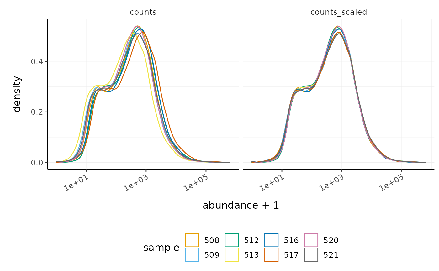
In this dataset the distributions of the counts are not very different to each other before scaling but scaling does make the distributions more similar. If we saw a sample with a very different distribution we may need to investigate it.
As tidybulk smoothly integrates with ggplot2 and other tidyverse packages it can save on typing and make plots easier to generate. Compare the code for creating density plots with tidybulk versus standard base R below (standard code adapted from (Law et al. 2016)).
tidybulk
# tidybulk
airway %>%
  tidybulk() %>%
  keep_abundant(factor_of_interest = dex) %>%
  scale_abundance() %>%
  pivot_longer(cols = c("counts", "counts_scaled"), names_to = "source", values_to = "abundance") %>%
  ggplot(aes(x = abundance + 1, color = sample)) +
  geom_density() +
  facet_wrap(~source) +
  scale_x_log10() +
  custom_theme
base R using edgeR
# Example code, no need to run

# Prepare data set
library(edgeR)
dgList <- SE2DGEList(airway)
group <- factor(dgList$samples$dex)
keep.exprs <- filterByExpr(dgList, group = group)
dgList <- dgList[keep.exprs, , keep.lib.sizes = FALSE]
nsamples <- ncol(dgList)
logcounts <- log2(dgList$counts)

# Setup graphics
col <- RColorBrewer::brewer.pal(nsamples, "Paired")
par(mfrow = c(1, 2))

# Plot raw counts
plot(density(logcounts[, 1]), col = col[1], lwd = 2, ylim = c(0, 0.26), las = 2, main = "", xlab = "")
title(main = "Counts")
for (i in 2:nsamples) {
  den <- density(logcounts[, i])
  lines(den$x, den$y, col = col[i], lwd = 2)
}
legend("topright", legend = dgList$samples$Run, text.col = col, bty = "n")

# Plot scaled counts
dgList_norm <- calcNormFactors(dgList)
lcpm_n <- cpm(dgList_norm, log = TRUE)
plot(density(lcpm_n[, 1]), col = col[1], lwd = 2, ylim = c(0, 0.26), las = 2, main = "", xlab = "")
title("Counts scaled")
for (i in 2:nsamples) {
  den <- density(lcpm_n[, i])
  lines(den$x, den$y, col = col[i], lwd = 2)
}
legend("topright", legend = dgList_norm$samples$Run, text.col = col, bty = "n")
Exploratory analyses
Dimensionality reduction
By far, one of the most important plots we make when we analyse RNA sequencing data are principal-component analysis (PCA) or multi-dimensional scaling (MDS) plots. We reduce the dimensions of the data to identify the greatest sources of variation in the data. A principal components analysis is an example of an unsupervised analysis, where we don’t need to specify the groups. If your experiment is well controlled and has worked well, what we hope to see is that the greatest sources of variation in the data are the treatments/groups we are interested in. It is also an incredibly useful tool for quality control and checking for outliers. We can use the reduce_dimensions function to calculate the dimensions.
# Get principal components
counts_scal_PCA <-
  counts_scaled %>%
  reduce_dimensions(method = "PCA")
#> Getting the 500 most variable genes
#> Fraction of variance explained by the selected principal components
#> # A tibble: 2 x 2
#>   `Fraction of variance`    PC
#>                    <dbl> <int>
#> 1                  0.353     1
#> 2                  0.312     2
#> tidybulk says: to access the raw results do `attr(..., "internals")$PCA`
This joins the result to the counts object.
# Take a look
counts_scal_PCA
#> # A tibble: 127,408 x 19
#>    feature sample counts SampleName cell  dex   albut Run   avgLength Experiment
#>    <fct>   <chr>   <int> <fct>      <fct> <fct> <fct> <fct>     <int> <fct>
#>  1 ENSG00… 508       679 GSM1275862 N613… untrt untrt SRR1…       126 SRX384345
#>  2 ENSG00… 508       467 GSM1275862 N613… untrt untrt SRR1…       126 SRX384345
#>  3 ENSG00… 508       260 GSM1275862 N613… untrt untrt SRR1…       126 SRX384345
#>  4 ENSG00… 508        60 GSM1275862 N613… untrt untrt SRR1…       126 SRX384345
#>  5 ENSG00… 508      3251 GSM1275862 N613… untrt untrt SRR1…       126 SRX384345
#>  6 ENSG00… 508      1433 GSM1275862 N613… untrt untrt SRR1…       126 SRX384345
#>  7 ENSG00… 508       519 GSM1275862 N613… untrt untrt SRR1…       126 SRX384345
#>  8 ENSG00… 508       394 GSM1275862 N613… untrt untrt SRR1…       126 SRX384345
#>  9 ENSG00… 508       172 GSM1275862 N613… untrt untrt SRR1…       126 SRX384345
#> 10 ENSG00… 508      2112 GSM1275862 N613… untrt untrt SRR1…       126 SRX384345
#> # … with 127,398 more rows, and 9 more variables: Sample <fct>,
#> #   BioSample <fct>, symbol <chr>, .abundant <lgl>, TMM <dbl>,
#> #   multiplier <dbl>, counts_scaled <dbl>, PC1 <dbl>, PC2 <dbl>
For plotting, we can select just the sample-wise information with pivot_sample.
# take a look
counts_scal_PCA %>% pivot_sample()
#> # A tibble: 8 x 15
#>   sample SampleName cell  dex   albut Run   avgLength Experiment Sample
#>   <chr>  <fct>      <fct> <fct> <fct> <fct>     <int> <fct>      <fct>
#> 1 508    GSM1275862 N613… untrt untrt SRR1…       126 SRX384345  SRS50…
#> 2 509    GSM1275863 N613… trt   untrt SRR1…       126 SRX384346  SRS50…
#> 3 512    GSM1275866 N052… untrt untrt SRR1…       126 SRX384349  SRS50…
#> 4 513    GSM1275867 N052… trt   untrt SRR1…        87 SRX384350  SRS50…
#> 5 516    GSM1275870 N080… untrt untrt SRR1…       120 SRX384353  SRS50…
#> 6 517    GSM1275871 N080… trt   untrt SRR1…       126 SRX384354  SRS50…
#> 7 520    GSM1275874 N061… untrt untrt SRR1…       101 SRX384357  SRS50…
#> 8 521    GSM1275875 N061… trt   untrt SRR1…        98 SRX384358  SRS50…
#> # … with 6 more variables: BioSample <fct>, .abundant <lgl>, TMM <dbl>,
#> #   multiplier <dbl>, PC1 <dbl>, PC2 <dbl>
We can now plot the reduced dimensions.
# PCA plot
counts_scal_PCA %>%
  pivot_sample() %>%
  ggplot(aes(x = PC1, y = PC2, colour = dex, shape = cell)) +
  geom_point() +
  geom_text_repel(aes(label = sample), show.legend = FALSE) +
  custom_theme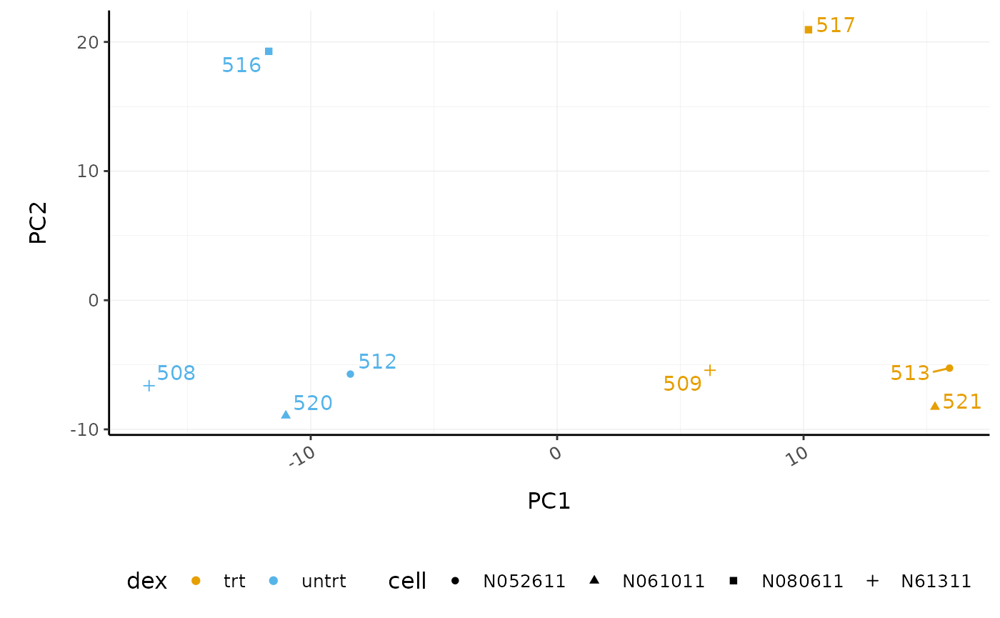
The samples separate by treatment on PC1 which is what we hope to see. PC2 separates the N080611 cell line from the other samples, indicating a greater difference between that cell line and the others.
Hierarchical clustering with heatmaps
An alternative to principal component analysis for examining relationships between samples is using hierarchical clustering. Heatmaps are a nice visualisation to examine hierarchical clustering of your samples. tidybulk has a simple function we can use, keep_variable, to extract the most variable genes which we can then plot with tidyHeatmap.
counts_scal_PCA %>%

  # extract 500 most variable genes
  keep_variable(.abundance = counts_scaled, top = 500) %>%

  # create heatmap
  heatmap(
    .column = sample,
    .row = feature,
    .value = counts_scaled,
    transform = log1p
  ) %>%
  add_tile(dex) %>%
  add_tile(cell)
#> Getting the 500 most variable genes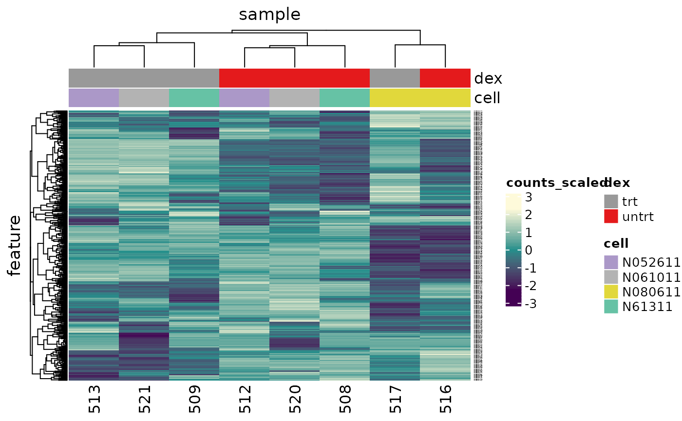
In the heatmap we can see the samples cluster into two groups, treated and untreated, for three of the cell lines, and the cell line (N080611) again is further away from the others.
Tidybulk enables a simplified way of generating a clustered heatmap of variable genes. Compare the code below for tidybulk versus a base R method.
base R using edgeR
# Example code, no need to run

library(edgeR)
dgList <- SE2DGEList(airway)
group <- factor(dgList$samples$dex)
keep.exprs <- filterByExpr(dgList, group = group)
dgList <- dgList[keep.exprs, , keep.lib.sizes = FALSE]
dgList <- calcNormFactors(dgList)
logcounts <- cpm(dgList, log = TRUE)
var_genes <- apply(logcounts, 1, var)
select_var <- names(sort(var_genes, decreasing = TRUE))[1:500]
highly_variable_lcpm <- logcounts[select_var, ]
colours <- c("#440154FF", "#21908CFF", "#fefada")
col.group <- c("red", "grey")[group]
gplots::heatmap.2(highly_variable_lcpm, col = colours, trace = "none", ColSideColors = col.group, scale = "row")
Differential expression
tidybulk integrates several popular methods for differential transcript abundance testing: the edgeR quasi-likelihood (Chen, Lun, and Smyth 2016) (tidybulk default method), edgeR likelihood ratio (McCarthy, Chen, and Smyth 2012), limma-voom (Law et al. 2014) and DESeq2 (Love, Huber, and Anders 2014). A common question researchers have is which method to choose. With tidybulk we can easily run multiple methods and compare.
We give test_differential_abundance our tidybulk counts object and a formula, specifying the column that contains our groups to be compared. If all our samples were from the same cell line, and there were no additional factors contributing variance such as batch differences, we could use the formula ~ dex. However, each treated and untreated sample is from a different cell line so we add the cell line as an additional factor ~ dex + cell.
de_all <-

  counts_scal_PCA %>%

  # edgeR QLT
  test_differential_abundance(
    ~ dex + cell,
    method = "edgeR_quasi_likelihood",
    prefix = "edgerQLT_"
  ) %>%

  # edgeR LRT
  test_differential_abundance(
    ~ dex + cell,
    method = "edgeR_likelihood_ratio",
    prefix = "edgerLR_"
  ) %>%

  # limma-voom
  test_differential_abundance(
    ~ dex + cell,
    method = "limma_voom",
    prefix = "voom_"
  ) %>%

  # DESeq2
  test_differential_abundance(
    ~ dex + cell,
    method = "deseq2",
    prefix = "deseq2_"
  )

# take a look

de_all
#> # A tibble: 127,408 x 41
#>    feature sample counts SampleName cell  dex   albut Run   avgLength Experiment
#>    <chr>   <chr>   <int> <fct>      <fct> <fct> <fct> <fct>     <int> <fct>
#>  1 ENSG00… 508       679 GSM1275862 N613… untrt untrt SRR1…       126 SRX384345
#>  2 ENSG00… 508       467 GSM1275862 N613… untrt untrt SRR1…       126 SRX384345
#>  3 ENSG00… 508       260 GSM1275862 N613… untrt untrt SRR1…       126 SRX384345
#>  4 ENSG00… 508        60 GSM1275862 N613… untrt untrt SRR1…       126 SRX384345
#>  5 ENSG00… 508      3251 GSM1275862 N613… untrt untrt SRR1…       126 SRX384345
#>  6 ENSG00… 508      1433 GSM1275862 N613… untrt untrt SRR1…       126 SRX384345
#>  7 ENSG00… 508       519 GSM1275862 N613… untrt untrt SRR1…       126 SRX384345
#>  8 ENSG00… 508       394 GSM1275862 N613… untrt untrt SRR1…       126 SRX384345
#>  9 ENSG00… 508       172 GSM1275862 N613… untrt untrt SRR1…       126 SRX384345
#> 10 ENSG00… 508      2112 GSM1275862 N613… untrt untrt SRR1…       126 SRX384345
#> # … with 127,398 more rows, and 31 more variables: Sample <fct>,
#> #   BioSample <fct>, symbol <chr>, .abundant <lgl>, TMM <dbl>,
#> #   multiplier <dbl>, counts_scaled <dbl>, PC1 <dbl>, PC2 <dbl>,
#> #   edgerQLT_logFC <dbl>, edgerQLT_logCPM <dbl>, edgerQLT_F <dbl>,
#> #   edgerQLT_PValue <dbl>, edgerQLT_FDR <dbl>, edgerLR_logFC <dbl>,
#> #   edgerLR_logCPM <dbl>, edgerLR_LR <dbl>, edgerLR_PValue <dbl>,
#> #   edgerLR_FDR <dbl>, voom_logFC <dbl>, voom_AveExpr <dbl>, voom_t <dbl>,
#> #   voom_P.Value <dbl>, voom_adj.P.Val <dbl>, voom_B <dbl>,
#> #   deseq2_baseMean <dbl>, deseq2_log2FoldChange <dbl>, deseq2_lfcSE <dbl>,
#> #   deseq2_stat <dbl>, deseq2_pvalue <dbl>, deseq2_padj <dbl>
This outputs the columns from each method such as log-fold change (logFC), false-discovery rate (FDR) and probability value (p-value). logFC is log2(treated/untreated).
Comparison of methods
We can visually compare the significance for all methods. We will notice that there is some difference between the methods.
de_all %>%
  pivot_transcript() %>%
  select(edgerQLT_PValue, edgerLR_PValue, voom_P.Value, deseq2_pvalue, feature) %>%
  ggpairs(1:4)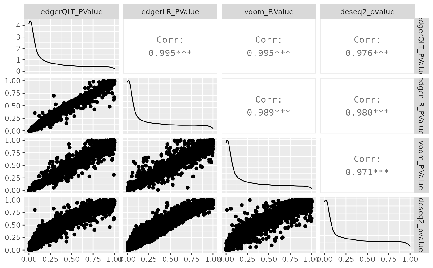
In order to decide which genes are differentially expressed, we usually take a cut-off of 0.05 on the FDR (or adjusted P value), NOT the raw p-value. This is because we are testing many genes (multiple testing), and the chances of finding differentially expressed genes is very high when you do that many tests. Hence we need to control the false discovery rate, which is the adjusted p-value column in the results table. What this means is that if 100 genes are significant at a 5% false discovery rate, we are willing to accept that 5 will be false positives.
We can count how many differentially expressed genes there are, for example with the edgeR QLT method. We’ll filter on FDR 0.05.
de_all %>%
  filter(edgerQLT_FDR < 0.05) %>%
  summarise(num_de = n_distinct(feature))
#> # A tibble: 1 x 1
#>   num_de
#>    <int>
#> 1   4967
Single method
If we just wanted to run one differential testing method we could do that. The default method is edgeR quasi-likelihood.
counts_de <- counts_scal_PCA %>%
  test_differential_abundance(~ dex + cell)
#> =====================================
#> tidybulk says: All testing methods use raw counts, irrespective of if scale_abundance
#> or adjust_abundance have been calculated. Therefore, it is essential to add covariates
#> such as batch effects (if applicable) in the formula.
#> =====================================
#> tidybulk says: The design column names are "(Intercept), dexuntrt, cellN061011, cellN080611, cellN61311"
#> tidybulk says: to access the raw results (fitted GLM) do `attr(..., "internals")$edgeR`
Tidybulk enables a simplified way of performing an RNA sequencing differential expression analysis (with the benefit of smoothly integrating with ggplot2 and other tidyverse packages). Compare the code for a tidybulk edgeR analysis versus standard edgeR below.
standard edgeR
# Example code, no need to run

library(edgeR)
dgList <- SE2DGEList(airway)
group <- factor(dgList$samples$dex)
keep.exprs <- filterByExpr(dgList, group = group)
dgList <- dgList[keep.exprs, , keep.lib.sizes = FALSE]
dgList <- calcNormFactors(dgList)
cell <- factor(dgList$samples$cell)
design <- model.matrix(~ group + cell)
dgList <- estimateDisp(dgList, design)
fit <- glmQLFit(dgList, design)
qlf <- glmQLFTest(fit, coef=2)
Plots after testing for differentially expressed
Volcano plots
Volcano plots are a useful genome-wide plot for checking that the analysis looks good. Volcano plots enable us to visualise the significance of change (p-value) versus the fold change (logFC). Highly significant genes are towards the top of the plot. We can also colour significant genes (e.g. genes with false-discovery rate < 0.05)
# volcano plot, minimal
counts_de %>%
  ggplot(aes(x = logFC, y = PValue, colour = FDR < 0.05)) +
  geom_point() +
  scale_y_continuous(trans = "log10_reverse") +
  custom_theme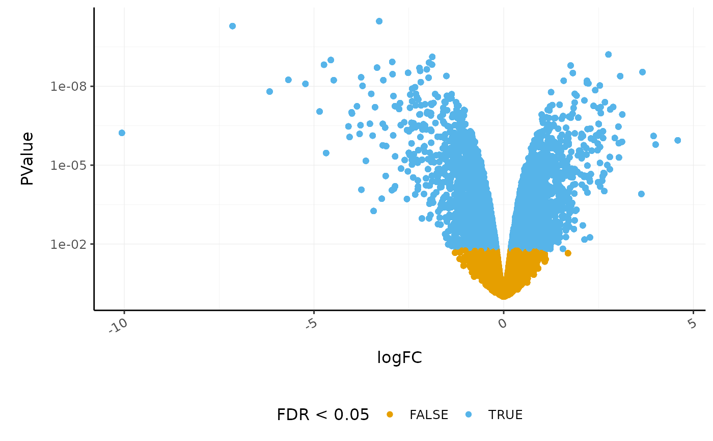
A more informative plot, integrating some of the packages in tidyverse.
We’ll extract the symbols for a few top genes (by P value) to use in some of the plots we will make.
topgenes_symbols <-
  counts_de %>%
  pivot_transcript() %>%
  arrange(PValue) %>%
  head(6) %>%
  pull(symbol)
counts_de %>%
  pivot_transcript() %>%

  # Subset data
  mutate(significant = FDR < 0.05 & abs(logFC) >= 2) %>%
  mutate(symbol = ifelse(symbol %in% topgenes_symbols, as.character(symbol), "")) %>%

  # Plot
  ggplot(aes(x = logFC, y = PValue, label = symbol)) +
  geom_point(aes(color = significant, size = significant, alpha = significant)) +
  geom_text_repel() +

  # Custom scales
  custom_theme +
  scale_y_continuous(trans = "log10_reverse") +
  scale_color_manual(values = c("black", "#e11f28")) +
  scale_size_discrete(range = c(0, 2))
#> Scale for 'colour' is already present. Adding another scale for 'colour',
#> which will replace the existing scale.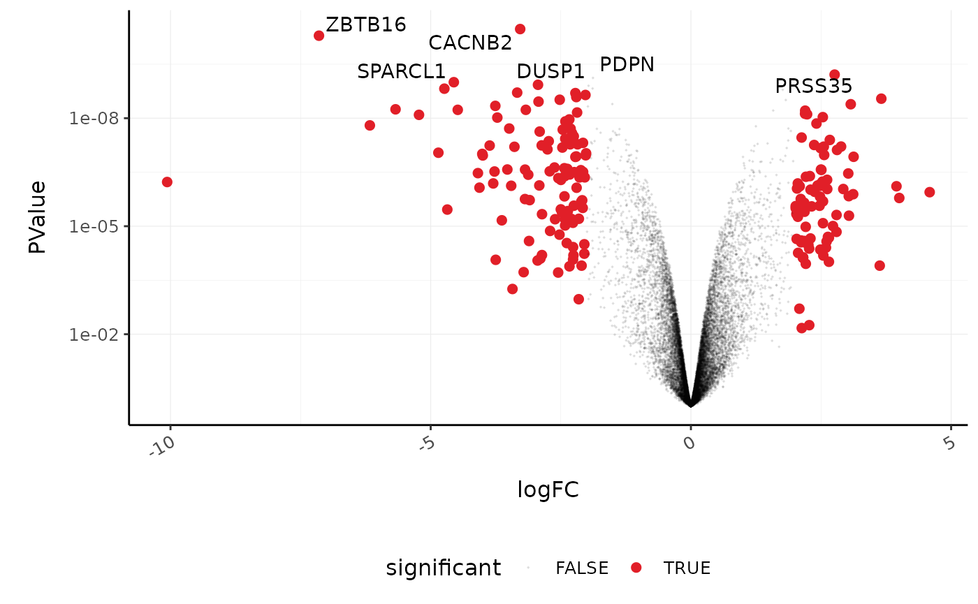
Automatic bibliography
Tidybulk provides a handy function called get_bibliography that keeps track of the references for the methods used in your tidybulk workflow. The references are in BibTeX format and can be imported into your reference manager.
get_bibliography(counts_de)
#> @article{robinson2010edger,
#>   title={edgeR: a Bioconductor package for differential expression analysis of digital gene expression data},
#>   author={Robinson, Mark D and McCarthy, Davis J and Smyth, Gordon K},
#>   journal={Bioinformatics},
#>   volume={26},
#>   number={1},
#>   pages={139--140},
#>   year={2010},
#>   publisher={Oxford University Press}
#>  }
#> @article{robinson2010scaling,
#>   title={A scaling normalization method for differential expression analysis of RNA-seq data},
#>   author={Robinson, Mark D and Oshlack, Alicia},
#>   journal={Genome biology},
#>   volume={11},
#>   number={3},
#>   pages={1--9},
#>   year={2010},
#>   publisher={BioMed Central}
#>  }
#>   @Manual{,
#>     title = {R: A Language and Environment for Statistical Computing},
#>     author = {{R Core Team}},
#>     organization = {R Foundation for Statistical Computing},
#>     address = {Vienna, Austria},
#>     year = {2020},
#>     url = {https://www.R-project.org/},
#>   }
#> @incollection{smyth2005limma,
#>   title={Limma: linear models for microarray data},
#>   author={Smyth, Gordon K},
#>   booktitle={Bioinformatics and computational biology solutions using R and Bioconductor},
#>   pages={397--420},
#>   year={2005},
#>   publisher={Springer}
#>  }
Cell type composition analysis
If we are sequencing tissue samples, we may want to know what cell types are present and if there are differences in expression between them. tidybulk has a deconvolve_cellularity function that can help us do this.
For this example we will use a subset of the breast cancer dataset from The Cancer Genome Atlas (TCGA).
BRCA_tidy <-
  bioceurope2020tidytranscriptomics::BRCA %>%
  tidybulk(patient, transcript, count)

BRCA_tidy
#> # A tibble: 198,374 x 5
#>    patient      transcript count  time event_occurred
#>    <fct>        <fct>      <int> <dbl>          <int>
#>  1 TCGA-C8-A275 C1orf112    1571     1              0
#>  2 TCGA-C8-A275 FGR         1873     1              0
#>  3 TCGA-C8-A275 FUCA2       3770     1              0
#>  4 TCGA-C8-A275 GCLC        2738     1              0
#>  5 TCGA-C8-A275 LAS1L       3175     1              0
#>  6 TCGA-C8-A275 ENPP4       1340     1              0
#>  7 TCGA-C8-A275 SEMA3F      5479     1              0
#>  8 TCGA-C8-A275 RAD52        472     1              0
#>  9 TCGA-C8-A275 BAD         1761     1              0
#> 10 TCGA-C8-A275 CD99       14697     1              0
#> # … with 198,364 more rows
With tidybulk, we can easily infer the proportions of cell types within a tissue using one of several published methods (Cibersort (Newman et al. 2015), EPIC (Racle et al. 2017) and llsr (Abbas et al. 2009)). Here we will use Cibersort which provides a default signature called LM22 to define the cell types. LM22 contains 547 genes that identify 22 human immune cell types.
BRCA_cell_type <-
  BRCA_tidy %>%
  deconvolve_cellularity(action = "get", cores = 1)

BRCA_cell_type
#> # A tibble: 22 x 25
#>    patient  time event_occurred `cibersort: B c… `cibersort: B c…
#>    <chr>   <dbl>          <int>            <dbl>            <dbl>
#>  1 TCGA-C…     1              0          0.0325            0
#>  2 TCGA-A…     1              0          0.0170            0
#>  3 TCGA-A…     5              0          0.00127           0
#>  4 TCGA-C…     5              0          0.0372            0
#>  5 TCGA-P…     5              0          0.00453           0
#>  6 TCGA-B…  6292              0          0.144             0
#>  7 TCGA-B…  7106              0          0.0632            0
#>  8 TCGA-B…  7777              0          0                 0.0142
#>  9 TCGA-B…  8008              0          0.203             0
#> 10 TCGA-B…  8391              0          0.147             0
#> # … with 12 more rows, and 20 more variables: `cibersort: Plasma cells` <dbl>,
#> #   `cibersort: T cells CD8` <dbl>, `cibersort: T cells CD4 naive` <dbl>,
#> #   `cibersort: T cells CD4 memory resting` <dbl>, `cibersort: T cells CD4
#> #   memory activated` <dbl>, `cibersort: T cells follicular helper` <dbl>,
#> #   `cibersort: T cells regulatory (Tregs)` <dbl>, `cibersort: T cells gamma
#> #   delta` <dbl>, `cibersort: NK cells resting` <dbl>, `cibersort: NK cells
#> #   activated` <dbl>, `cibersort: Monocytes` <dbl>, `cibersort: Macrophages
#> #   M0` <dbl>, `cibersort: Macrophages M1` <dbl>, `cibersort: Macrophages
#> #   M2` <dbl>, `cibersort: Dendritic cells resting` <dbl>, `cibersort:
#> #   Dendritic cells activated` <dbl>, `cibersort: Mast cells resting` <dbl>,
#> #   `cibersort: Mast cells activated` <dbl>, `cibersort: Eosinophils` <dbl>,
#> #   `cibersort: Neutrophils` <dbl>
Cell type proportions are added to the tibble as new columns. The prefix makes it easy to reshape the data frame if needed, for visualisation or further analyses.
BRCA_cell_type_long <-
  BRCA_cell_type %>%

  # Reshape
  pivot_longer(
    contains("cibersort"),
    names_prefix = "cibersort: ",
    names_to = "cell_type",
    values_to = "proportion"
  )

BRCA_cell_type_long
#> # A tibble: 484 x 5
#>    patient       time event_occurred cell_type                    proportion
#>    <chr>        <dbl>          <int> <chr>                             <dbl>
#>  1 TCGA-C8-A275     1              0 B cells naive                    0.0325
#>  2 TCGA-C8-A275     1              0 B cells memory                   0
#>  3 TCGA-C8-A275     1              0 Plasma cells                     0.0127
#>  4 TCGA-C8-A275     1              0 T cells CD8                      0
#>  5 TCGA-C8-A275     1              0 T cells CD4 naive                0.0507
#>  6 TCGA-C8-A275     1              0 T cells CD4 memory resting       0.0299
#>  7 TCGA-C8-A275     1              0 T cells CD4 memory activated     0.0332
#>  8 TCGA-C8-A275     1              0 T cells follicular helper        0
#>  9 TCGA-C8-A275     1              0 T cells regulatory (Tregs)       0.0326
#> 10 TCGA-C8-A275     1              0 T cells gamma delta              0.0247
#> # … with 474 more rows
We can plot the proportions of immune cell types for each patient.
BRCA_cell_type_long %>%

  # Plot proportions
  ggplot(aes(x = patient, y = proportion, fill = cell_type)) +
  geom_bar(stat = "identity") +
  custom_theme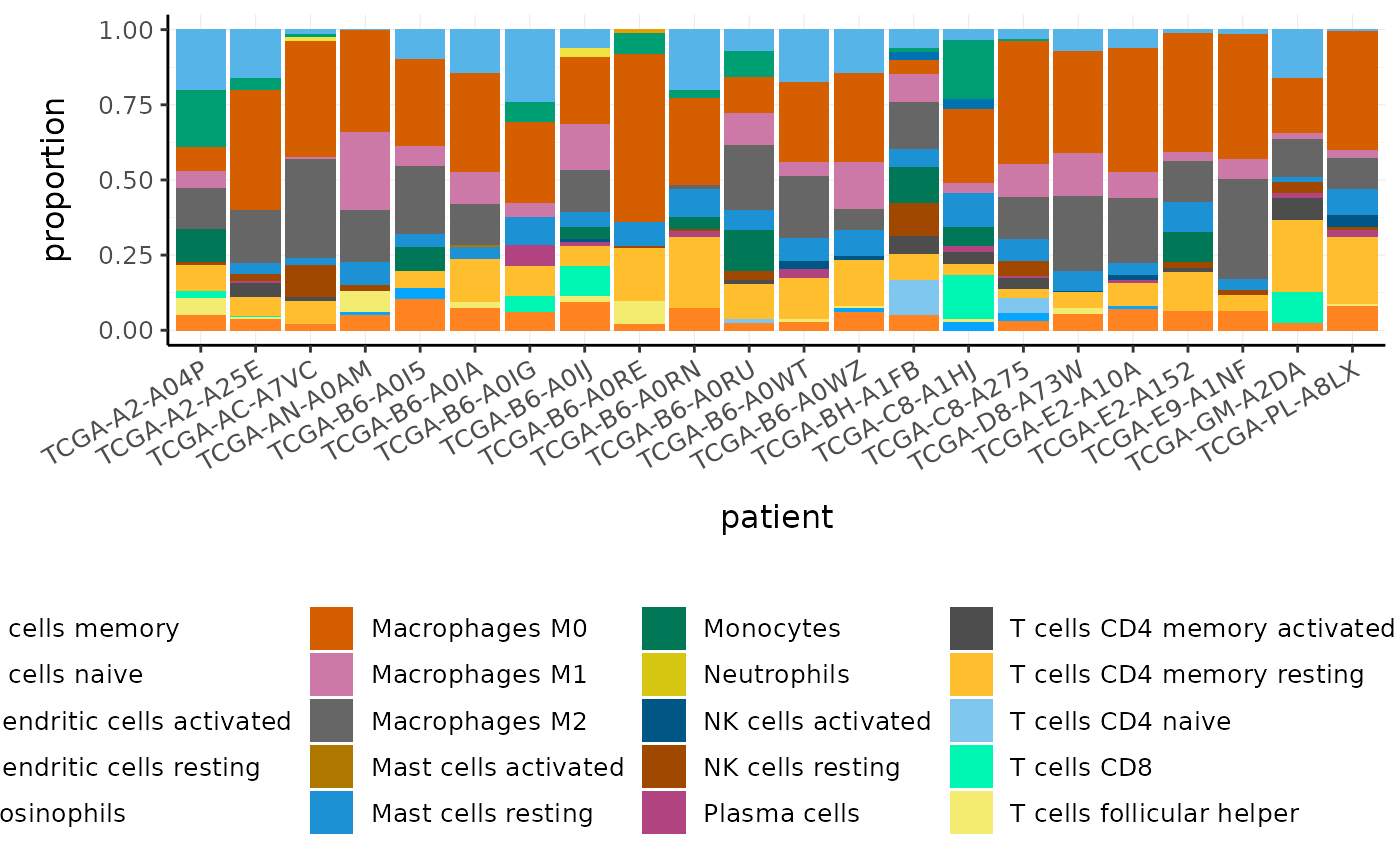
We can visualise the similarity of the tissue composition for the patients by performing a dimensionality reduction on cell type and proportion (rather than on transcript and counts as we did previously).
BRCA_cell_type_long %>%

  # Filter cell types with proportion zero in all patients
  group_by(cell_type) %>%
  filter(sum(proportion) > 0) %>%
  ungroup() %>%
  reduce_dimensions(
    patient,
    cell_type,
    proportion,
    method = "PCA",
    action = "get"
  ) %>%
  ggplot(aes(PC1, PC2, label = patient)) +
  geom_point(color = "red") +
  ggrepel::geom_text_repel(size = 3) +
  custom_theme
#> Getting the 21 most variable genes
#> Fraction of variance explained by the selected principal components
#> # A tibble: 2 x 2
#>   `Fraction of variance`    PC
#>                    <dbl> <int>
#> 1                  0.183     1
#> 2                  0.152     2
#> tidybulk says: to access the raw results do `attr(..., "internals")$PCA`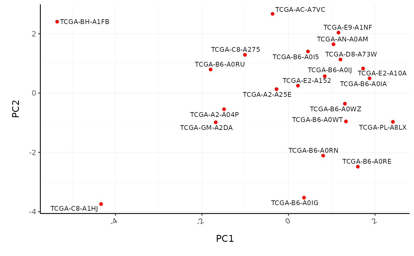
Key Points
- RNA sequencing data can be represented and analysed in a ‘tidy’ way using tidybulk and the tidyverse
- With the modularity offered by piping we don’t need to create variables, unless an object is used more than one. This improves robustness of the code.
- The principles of tidy transcriptomics are to interface as much as possible with commonly known manipulation and visualisation tools, rather than creating custom functions.
- Some of the key steps in an RNA sequencing analysis are (i) filtering lowly abundant transcripts, (ii) adjusting for differences in sequencing depth and composition, (iii) testing for differential expression
- Dimensionality reduction (PCA or MDS) plots are very important for exploring the data
- Density plots, volcano plots, strip-charts and heatmaps are useful visualisation tools for evaluating the hypothesis testing.
-
tidybulkallows streamlined multi-method analyses -
tidybulkallow easy analyses of cell type composition - Testing for differences in tissue composition between samples is analogous to the testing for differences in transcript abundance
Supplementary
Some things we don’t have time to cover in Part 1 of this workshop can be found in the Supplementary material.
Part 2 Bulk RNA-seq with tidySummarizedExperiment and Bioconductor
Tidify SummarizedExperiment into tidySummarizedExperiment
This is a SummarizedExperiment object but it is evaluated as tibble. So it is fully compatible both with SummarizedExperiment and tidyverse APIs.
library(tidySummarizedExperiment)
#>
#> Attaching package: 'tidySummarizedExperiment'
#> The following objects are masked from 'package:tidybulk':
#>
#>     bind_cols, bind_rows, distinct, filter, full_join, group_by,
#>     inner_join, left_join, mutate, nest, rename, right_join, rowwise,
#>     summarise, unnest
#> The following object is masked from 'package:tidyHeatmap':
#>
#>     pasilla
#> The following object is masked from 'package:plotly':
#>
#>     plot_ly
#> The following objects are masked from 'package:dplyr':
#>
#>     bind_cols, bind_rows, count
#> The following object is masked from 'package:IRanges':
#>
#>     slice
#> The following object is masked from 'package:S4Vectors':
#>
#>     rename
#> The following object is masked from 'package:matrixStats':
#>
#>     count
#> The following object is masked from 'package:stats':
#>
#>     filter
pasilla_tidy <- airway %>% tidy()
It looks like a tibble
pasilla_tidy
#> # A tibble abstraction: 512,816 x 21
#>    sample SampleName cell  dex   albut Run   avgLength Experiment Sample
#>    <chr>  <fct>      <fct> <fct> <fct> <fct>     <int> <fct>      <fct>
#>  1 SRR10… GSM1275862 N613… untrt untrt SRR1…       126 SRX384345  SRS50…
#>  2 SRR10… GSM1275862 N613… untrt untrt SRR1…       126 SRX384345  SRS50…
#>  3 SRR10… GSM1275862 N613… untrt untrt SRR1…       126 SRX384345  SRS50…
#>  4 SRR10… GSM1275862 N613… untrt untrt SRR1…       126 SRX384345  SRS50…
#>  5 SRR10… GSM1275862 N613… untrt untrt SRR1…       126 SRX384345  SRS50…
#>  6 SRR10… GSM1275862 N613… untrt untrt SRR1…       126 SRX384345  SRS50…
#>  7 SRR10… GSM1275862 N613… untrt untrt SRR1…       126 SRX384345  SRS50…
#>  8 SRR10… GSM1275862 N613… untrt untrt SRR1…       126 SRX384345  SRS50…
#>  9 SRR10… GSM1275862 N613… untrt untrt SRR1…       126 SRX384345  SRS50…
#> 10 SRR10… GSM1275862 N613… untrt untrt SRR1…       126 SRX384345  SRS50…
#> # … with 40 more rows, and 12 more variables: BioSample <fct>,
#> #   transcript <chr>, counts <int>, group <int>, group_name <chr>,
#> #   seqnames <fct>, start <int>, end <int>, width <int>, strand <fct>,
#> #   exon_id <int>, exon_name <chr>
But it is a SummarizedExperiment object after all
assays(pasilla_tidy)
#> List of length 1
#> names(1): counts
Tidyverse commands
We can use tidyverse commands to explore the tidy SummarizedExperiment object.
We can use slice to choose rows by position, for example to choose the first row.
pasilla_tidy %>% slice(1)
#> # A tibble abstraction: 1 x 21
#>   sample SampleName cell  dex   albut Run   avgLength Experiment Sample
#>   <chr>  <fct>      <fct> <fct> <fct> <fct>     <int> <fct>      <fct>
#> 1 SRR10… GSM1275862 N613… untrt untrt SRR1…       126 SRX384345  SRS50…
#> # … with 12 more variables: BioSample <fct>, transcript <chr>, counts <int>,
#> #   group <int>, group_name <chr>, seqnames <fct>, start <int>, end <int>,
#> #   width <int>, strand <fct>, exon_id <int>, exon_name <chr>
We can use filter to choose rows by criteria.
pasilla_tidy %>% filter(dex == "untrt")
#> # A tibble abstraction: 256,408 x 21
#>    sample SampleName cell  dex   albut Run   avgLength Experiment Sample
#>    <chr>  <fct>      <fct> <fct> <fct> <fct>     <int> <fct>      <fct>
#>  1 SRR10… GSM1275862 N613… untrt untrt SRR1…       126 SRX384345  SRS50…
#>  2 SRR10… GSM1275862 N613… untrt untrt SRR1…       126 SRX384345  SRS50…
#>  3 SRR10… GSM1275862 N613… untrt untrt SRR1…       126 SRX384345  SRS50…
#>  4 SRR10… GSM1275862 N613… untrt untrt SRR1…       126 SRX384345  SRS50…
#>  5 SRR10… GSM1275862 N613… untrt untrt SRR1…       126 SRX384345  SRS50…
#>  6 SRR10… GSM1275862 N613… untrt untrt SRR1…       126 SRX384345  SRS50…
#>  7 SRR10… GSM1275862 N613… untrt untrt SRR1…       126 SRX384345  SRS50…
#>  8 SRR10… GSM1275862 N613… untrt untrt SRR1…       126 SRX384345  SRS50…
#>  9 SRR10… GSM1275862 N613… untrt untrt SRR1…       126 SRX384345  SRS50…
#> 10 SRR10… GSM1275862 N613… untrt untrt SRR1…       126 SRX384345  SRS50…
#> # … with 40 more rows, and 12 more variables: BioSample <fct>,
#> #   transcript <chr>, counts <int>, group <int>, group_name <chr>,
#> #   seqnames <fct>, start <int>, end <int>, width <int>, strand <fct>,
#> #   exon_id <int>, exon_name <chr>
We can use select to choose columns.
pasilla_tidy %>% select(sample)
#> tidySummarizedExperiment says: Key columns are missing. A data frame is returned for independent data analysis.
#> # A tibble: 512,816 x 1
#>    sample
#>    <chr>
#>  1 SRR1039508
#>  2 SRR1039508
#>  3 SRR1039508
#>  4 SRR1039508
#>  5 SRR1039508
#>  6 SRR1039508
#>  7 SRR1039508
#>  8 SRR1039508
#>  9 SRR1039508
#> 10 SRR1039508
#> # … with 512,806 more rows
We can use count to count how many rows we have for each sample.
pasilla_tidy %>% count(sample)
#> tidySummarizedExperiment says: A data frame is returned for independent data analysis.
#> # A tibble: 8 x 2
#>   sample         n
#>   <chr>      <int>
#> 1 SRR1039508 64102
#> 2 SRR1039509 64102
#> 3 SRR1039512 64102
#> 4 SRR1039513 64102
#> 5 SRR1039516 64102
#> 6 SRR1039517 64102
#> 7 SRR1039520 64102
#> 8 SRR1039521 64102
We can use distinct to see what distinct sample information we have.
pasilla_tidy %>% distinct(sample, dex, cell)
#> tidySummarizedExperiment says: A data frame is returned for independent data analysis.
#> # A tibble: 8 x 3
#>   sample     cell    dex
#>   <chr>      <fct>   <fct>
#> 1 SRR1039508 N61311  untrt
#> 2 SRR1039509 N61311  trt
#> 3 SRR1039512 N052611 untrt
#> 4 SRR1039513 N052611 trt
#> 5 SRR1039516 N080611 untrt
#> 6 SRR1039517 N080611 trt
#> 7 SRR1039520 N061011 untrt
#> 8 SRR1039521 N061011 trt
We could use rename to rename a column. For example, to modify the type column name.
pasilla_tidy %>% rename(treatment_status=dex)
#> # A tibble abstraction: 512,816 x 21
#>    sample SampleName cell  treatment_status albut Run   avgLength Experiment
#>    <chr>  <fct>      <fct> <fct>            <fct> <fct>     <int> <fct>
#>  1 SRR10… GSM1275862 N613… untrt            untrt SRR1…       126 SRX384345
#>  2 SRR10… GSM1275862 N613… untrt            untrt SRR1…       126 SRX384345
#>  3 SRR10… GSM1275862 N613… untrt            untrt SRR1…       126 SRX384345
#>  4 SRR10… GSM1275862 N613… untrt            untrt SRR1…       126 SRX384345
#>  5 SRR10… GSM1275862 N613… untrt            untrt SRR1…       126 SRX384345
#>  6 SRR10… GSM1275862 N613… untrt            untrt SRR1…       126 SRX384345
#>  7 SRR10… GSM1275862 N613… untrt            untrt SRR1…       126 SRX384345
#>  8 SRR10… GSM1275862 N613… untrt            untrt SRR1…       126 SRX384345
#>  9 SRR10… GSM1275862 N613… untrt            untrt SRR1…       126 SRX384345
#> 10 SRR10… GSM1275862 N613… untrt            untrt SRR1…       126 SRX384345
#> # … with 40 more rows, and 13 more variables: Sample <fct>, BioSample <fct>,
#> #   transcript <chr>, counts <int>, group <int>, group_name <chr>,
#> #   seqnames <fct>, start <int>, end <int>, width <int>, strand <fct>,
#> #   exon_id <int>, exon_name <chr>
We could use mutate to create a column. For example, we could create a new type column that contains single and paired instead of single_end and paired_end.
pasilla_tidy %>% mutate(type=str_remove(sample, "SRR1039"))
#> # A tibble abstraction: 512,816 x 22
#>    sample SampleName cell  dex   albut Run   avgLength Experiment Sample
#>    <chr>  <fct>      <fct> <fct> <fct> <fct>     <int> <fct>      <fct>
#>  1 SRR10… GSM1275862 N613… untrt untrt SRR1…       126 SRX384345  SRS50…
#>  2 SRR10… GSM1275862 N613… untrt untrt SRR1…       126 SRX384345  SRS50…
#>  3 SRR10… GSM1275862 N613… untrt untrt SRR1…       126 SRX384345  SRS50…
#>  4 SRR10… GSM1275862 N613… untrt untrt SRR1…       126 SRX384345  SRS50…
#>  5 SRR10… GSM1275862 N613… untrt untrt SRR1…       126 SRX384345  SRS50…
#>  6 SRR10… GSM1275862 N613… untrt untrt SRR1…       126 SRX384345  SRS50…
#>  7 SRR10… GSM1275862 N613… untrt untrt SRR1…       126 SRX384345  SRS50…
#>  8 SRR10… GSM1275862 N613… untrt untrt SRR1…       126 SRX384345  SRS50…
#>  9 SRR10… GSM1275862 N613… untrt untrt SRR1…       126 SRX384345  SRS50…
#> 10 SRR10… GSM1275862 N613… untrt untrt SRR1…       126 SRX384345  SRS50…
#> # … with 40 more rows, and 13 more variables: BioSample <fct>, type <chr>,
#> #   transcript <chr>, counts <int>, group <int>, group_name <chr>,
#> #   seqnames <fct>, start <int>, end <int>, width <int>, strand <fct>,
#> #   exon_id <int>, exon_name <chr>
We could use unite to combine multiple columns into a single column.
pasilla_tidy %>% unite("combined", c(dex, cell))
#> # A tibble abstraction: 512,816 x 20
#>    sample SampleName combined albut Run   avgLength Experiment Sample BioSample
#>    <chr>  <fct>      <chr>    <fct> <fct>     <int> <fct>      <fct>  <fct>
#>  1 SRR10… GSM1275862 untrt_N… untrt SRR1…       126 SRX384345  SRS50… SAMN0242…
#>  2 SRR10… GSM1275862 untrt_N… untrt SRR1…       126 SRX384345  SRS50… SAMN0242…
#>  3 SRR10… GSM1275862 untrt_N… untrt SRR1…       126 SRX384345  SRS50… SAMN0242…
#>  4 SRR10… GSM1275862 untrt_N… untrt SRR1…       126 SRX384345  SRS50… SAMN0242…
#>  5 SRR10… GSM1275862 untrt_N… untrt SRR1…       126 SRX384345  SRS50… SAMN0242…
#>  6 SRR10… GSM1275862 untrt_N… untrt SRR1…       126 SRX384345  SRS50… SAMN0242…
#>  7 SRR10… GSM1275862 untrt_N… untrt SRR1…       126 SRX384345  SRS50… SAMN0242…
#>  8 SRR10… GSM1275862 untrt_N… untrt SRR1…       126 SRX384345  SRS50… SAMN0242…
#>  9 SRR10… GSM1275862 untrt_N… untrt SRR1…       126 SRX384345  SRS50… SAMN0242…
#> 10 SRR10… GSM1275862 untrt_N… untrt SRR1…       126 SRX384345  SRS50… SAMN0242…
#> # … with 40 more rows, and 11 more variables: transcript <chr>, counts <int>,
#> #   group <int>, group_name <chr>, seqnames <fct>, start <int>, end <int>,
#> #   width <int>, strand <fct>, exon_id <int>, exon_name <chr>
We can also combine commands with the tidyverse pipe %>%.
For example, we could combine group_by and summarise to get the total counts for each sample.
pasilla_tidy %>%
    group_by(sample) %>%
    summarise(total_counts=sum(counts))
#> tidySummarizedExperiment says: A data frame is returned for independent data analysis.
#> `summarise()` ungrouping output (override with `.groups` argument)
#> # A tibble: 8 x 2
#>   sample     total_counts
#>   <chr>             <int>
#> 1 SRR1039508     20637971
#> 2 SRR1039509     18809481
#> 3 SRR1039512     25348649
#> 4 SRR1039513     15163415
#> 5 SRR1039516     24448408
#> 6 SRR1039517     30818215
#> 7 SRR1039520     19126151
#> 8 SRR1039521     21164133
We could combine group_by, mutate and filter to get the transcripts with mean count > 0.
pasilla_tidy %>%
    group_by(seqnames ) %>%
    mutate(mean_count=mean(counts)) %>%
    filter(mean_count > 0)
#> tidySummarizedExperiment says: A data frame is returned for independent data analysis.
#> # A tibble: 512,816 x 22
#> # Groups:   seqnames [1]
#>    sample SampleName cell  dex   albut Run   avgLength Experiment Sample
#>    <chr>  <fct>      <fct> <fct> <fct> <fct>     <int> <fct>      <fct>
#>  1 SRR10… GSM1275862 N613… untrt untrt SRR1…       126 SRX384345  SRS50…
#>  2 SRR10… GSM1275862 N613… untrt untrt SRR1…       126 SRX384345  SRS50…
#>  3 SRR10… GSM1275862 N613… untrt untrt SRR1…       126 SRX384345  SRS50…
#>  4 SRR10… GSM1275862 N613… untrt untrt SRR1…       126 SRX384345  SRS50…
#>  5 SRR10… GSM1275862 N613… untrt untrt SRR1…       126 SRX384345  SRS50…
#>  6 SRR10… GSM1275862 N613… untrt untrt SRR1…       126 SRX384345  SRS50…
#>  7 SRR10… GSM1275862 N613… untrt untrt SRR1…       126 SRX384345  SRS50…
#>  8 SRR10… GSM1275862 N613… untrt untrt SRR1…       126 SRX384345  SRS50…
#>  9 SRR10… GSM1275862 N613… untrt untrt SRR1…       126 SRX384345  SRS50…
#> 10 SRR10… GSM1275862 N613… untrt untrt SRR1…       126 SRX384345  SRS50…
#> # … with 512,806 more rows, and 13 more variables: BioSample <fct>,
#> #   transcript <chr>, counts <int>, group <int>, group_name <chr>,
#> #   seqnames <fct>, start <int>, end <int>, width <int>, strand <fct>,
#> #   exon_id <int>, exon_name <chr>, mean_count <dbl>
Plotting
We can treat pasilla_tidy as a normal tibble for plotting. Here we plot the distribution of counts per sample.
pasilla_tidy %>%
    ggplot(aes(counts + 1, group=sample, color=`dex`)) +
    geom_density() +
    scale_x_log10() +
    custom_theme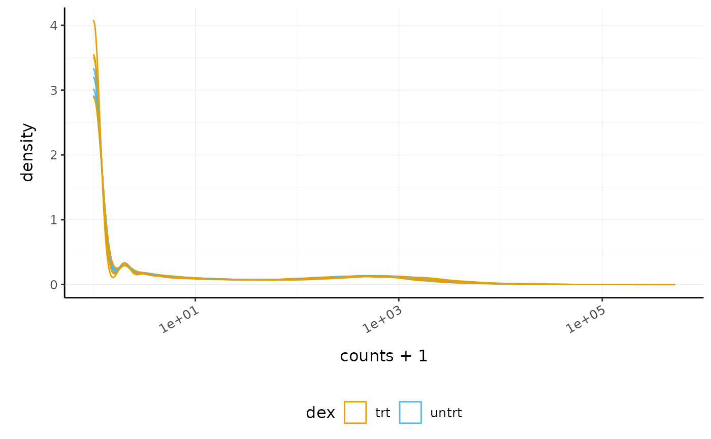
Part 3 Single-cell RNA-seq with tidySingleCellExperiment
In Part 1 we showed how we can study the cell-type composition of a biological sample using bulk RNA sequencing. Single cell sequencing enables a more direct estimation of cell-type composition and gives greater resolution. For bulk RNA sequencing we need to infer the cell types using the abundance of transcripts in the whole sample, with single-cell RNA sequencing we can directly measure the transcripts in each cell and then classify the cells into cell types.
Introduction to tidySingleCellExperiment
SingleCellExperiment is a very popular container of single cell RNA sequencing data.
tidySingleCellExperiment provides a bridge between the SingleCellExperiment single-cell package and the tidyverse. It creates an invisible layer that enables viewing the SingleCellExperiment object as a tidyverse tibble, and provides SingleCellExperiment-compatible dplyr, tidyr, ggplot and plotly functions.
# load additional libraries
library(bioceurope2020tidytranscriptomics)
library(dplyr)
library(ggplot2)
library(purrr)
library(stringr)
library(SummarizedExperiment)
library(SingleCellExperiment)
library(scater)
library(scran)
library(igraph)
library(batchelor)
library(SingleR)
library(scuttle)
library(EnsDb.Hsapiens.v86)
library(celldex)
library(ggbeeswarm)
library(tidySingleCellExperiment)
The single-cell RNA sequencing data used here is 3000 cells in total, subsetted from 20 samples from 10 peripheral blood mononuclear cell (pbmc) datasets. The datasets are from GSE115189/SRR7244582 (Freytag et al. 2018), SRR11038995 [Cai et al. (2020), SCP345 (singlecell.broadinstitute.org), SCP424 (Ding et al. 2020), SCP591 (Karagiannis et al. 2020) and 10x-derived 6K and 8K datasets (support.10xgenomics.com/).
Create tidySingleCellExperiment
This is a SingleCellExperiment object but it is evaluated as tibble. So it is fully compatible both with SingleCellExperiment and tidyverse APIs.
pbmc_tidy <- pbmc %>% tidy()It looks like a tibble
pbmc_tidy
#> # A tibble abstraction: 3,000 x 8
#>    cell    file      orig.ident nCount_RNA nFeature_RNA  S.Score G2M.Score ident
#>    <chr>   <chr>     <chr>           <dbl>        <int>    <dbl>     <dbl> <fct>
#>  1 CCAGTC… ../data/… SeuratPro…       3421          979 -5.42e-2  -0.0107  G1
#>  2 ATGAGC… ../data/… SeuratPro…       2752          898 -5.01e-2  -0.00416 G1
#>  3 TATGAA… ../data/… SeuratPro…       2114          937 -2.95e-5  -0.0229  G1
#>  4 CATATA… ../data/… SeuratPro…       3122         1086 -6.65e-2  -0.0488  G1
#>  5 GAGGCA… ../data/… SeuratPro…       2341          957 -3.74e-3   0.0241  G2M
#>  6 AGCTGC… ../data/… SeuratPro…       5472         1758 -5.88e-2   0.00241 G2M
#>  7 TGATTA… ../data/… SeuratPro…       1258          542 -2.51e-2  -0.0269  G1
#>  8 ACGAAG… ../data/… SeuratPro…       7683         1926 -1.33e-1  -0.116   G1
#>  9 CGGCAT… ../data/… SeuratPro…       3500         1092 -6.87e-2  -0.0622  G1
#> 10 ATAGCG… ../data/… SeuratPro…       3092          974 -1.24e-2  -0.0271  G1
#> # … with 2,990 more rows
But it is a SingleCellExperiment object after all
So it can be interacted with using SingleCellExperiment commands such as assayNames.
assayNames(pbmc_tidy) # from SummarizedExperiment
#> [1] "counts"    "logcounts"
Extract gene information
We can join transcript-wise information for independent analyses
pbmc_tidy %>%
  join_transcripts("CD3G")
#> tidySingleCellExperiment says: A data frame is returned for independent data analysis.
#> # A tibble: 3,000 x 11
#>    cell  transcript abundance_counts abundance_logco… file  orig.ident
#>    <chr> <chr>                 <dbl>            <dbl> <chr> <chr>
#>  1 CCAG… CD3G                      0                0 ../d… SeuratPro…
#>  2 ATGA… CD3G                      1                1 ../d… SeuratPro…
#>  3 TATG… CD3G                      0                0 ../d… SeuratPro…
#>  4 CATA… CD3G                      0                0 ../d… SeuratPro…
#>  5 GAGG… CD3G                      2                2 ../d… SeuratPro…
#>  6 AGCT… CD3G                      2                2 ../d… SeuratPro…
#>  7 TGAT… CD3G                      0                0 ../d… SeuratPro…
#>  8 ACGA… CD3G                      0                0 ../d… SeuratPro…
#>  9 CGGC… CD3G                      0                0 ../d… SeuratPro…
#> 10 ATAG… CD3G                      0                0 ../d… SeuratPro…
#> # … with 2,990 more rows, and 5 more variables: nCount_RNA <dbl>,
#> #   nFeature_RNA <int>, S.Score <dbl>, G2M.Score <dbl>, ident <fct>
Polish the data
We can also interact with our object as we do with any tidyverse tibble. In this case we want to polish an annotation column. We will extract the sample and dataset names from the file name column into separate columns.
pbmc_tidy <-
  pbmc_tidy %>%

  # Extract sample and group
  extract(file, "sample", "../data/([a-zA-Z0-9_]+)/outs.+", remove = FALSE) %>%

  # Extract data source
  extract(file, c("dataset", "groups"), "../data/([a-zA-Z0-9_]+)_([0-9])/outs.+")

pbmc_tidy
#> # A tibble abstraction: 3,000 x 10
#>    cell  dataset groups sample orig.ident nCount_RNA nFeature_RNA  S.Score
#>    <chr> <chr>   <chr>  <chr>  <chr>           <dbl>        <int>    <dbl>
#>  1 CCAG… GSE115… 1      GSE11… SeuratPro…       3421          979 -5.42e-2
#>  2 ATGA… GSE115… 2      GSE11… SeuratPro…       2752          898 -5.01e-2
#>  3 TATG… GSE115… 2      GSE11… SeuratPro…       2114          937 -2.95e-5
#>  4 CATA… GSE115… 1      GSE11… SeuratPro…       3122         1086 -6.65e-2
#>  5 GAGG… GSE115… 2      GSE11… SeuratPro…       2341          957 -3.74e-3
#>  6 AGCT… GSE115… 1      GSE11… SeuratPro…       5472         1758 -5.88e-2
#>  7 TGAT… GSE115… 1      GSE11… SeuratPro…       1258          542 -2.51e-2
#>  8 ACGA… GSE115… 1      GSE11… SeuratPro…       7683         1926 -1.33e-1
#>  9 CGGC… GSE115… 1      GSE11… SeuratPro…       3500         1092 -6.87e-2
#> 10 ATAG… GSE115… 1      GSE11… SeuratPro…       3092          974 -1.24e-2
#> # … with 2,990 more rows, and 2 more variables: G2M.Score <dbl>, ident <fct>
Quality control
A key quality control step performed in single cell analysis is assessment of the proportion of mitochondrial transcripts. A high mitochondrial count can indicate the cell is dead or dying and is thus poor quality. A powerful combination of tools we can use with tidySingleCellExperiment is tidyverse’s nest and map. This enables us to easily perform independent analyses on subsets of the data. For example, we can nest by dataset and use map to iterate the analysis of mitochondrial content across each dataset.
Nesting
my_tibble =
  tibble(
  label = c("a","a","a","a","a","b","b","b","b","b" ),
  value = 1:10
)

my_tibble
#> # A tibble: 10 x 2
#>    label value
#>    <chr> <int>
#>  1 a         1
#>  2 a         2
#>  3 a         3
#>  4 a         4
#>  5 a         5
#>  6 b         6
#>  7 b         7
#>  8 b         8
#>  9 b         9
#> 10 b        10

my_tibble_nested =
  my_tibble %>%
  nest(data = value)

my_tibble_nested
#> # A tibble: 2 x 2
#>   label data
#>   <chr> <list>
#> 1 a     <tibble [5 × 1]>
#> 2 b     <tibble [5 × 1]>

# Summarise
my_tibble_nested %>%
  mutate(average = map_dbl(data, ~ mean(.x$value)))
#> # A tibble: 2 x 3
#>   label data             average
#>   <chr> <list>             <dbl>
#> 1 a     <tibble [5 × 1]>       3
#> 2 b     <tibble [5 × 1]>       8

# Summarise + filter
my_tibble_nested %>%
  mutate(average = map_dbl(data, ~ mean(.x$value))) %>%
  filter(average == max(average)) %>%
  unnest(data)
#> # A tibble: 5 x 3
#>   label value average
#>   <chr> <int>   <dbl>
#> 1 b         6       8
#> 2 b         7       8
#> 3 b         8       8
#> 4 b         9       8
#> 5 b        10       8

# Summarise + update
my_tibble_nested %>%
  mutate(average = map_dbl(data, ~ mean(.x$value))) %>%
  mutate(data = map2(data, average, ~ .x - .y )) %>%
  unnest(data)
#> # A tibble: 10 x 3
#>    label value average
#>    <chr> <dbl>   <dbl>
#>  1 a        -2       3
#>  2 a        -1       3
#>  3 a         0       3
#>  4 a         1       3
#>  5 a         2       3
#>  6 b        -2       8
#>  7 b        -1       8
#>  8 b         0       8
#>  9 b         1       8
#> 10 b         2       8
# Get chromosomal location for gene symbols
location <- mapIds(
  EnsDb.Hsapiens.v86,
  keys = rownames(pbmc_tidy),
  column = "SEQNAME",
  keytype = "SYMBOL"
)
#> Warning: Unable to map 5313 of 51958 requested IDs.

pbmc_tidy <-
  pbmc_tidy %>%

  # Grouping - nesting by dataset
  nest(data = -dataset) %>%
  mutate(mitochondrion_info = map(
    data,
    ~ # Calculating mitochondrial statistics
      perCellQCMetrics(.x, subsets = list(Mito = which(location == "MT"))) %>%

      # Converting to tibble
      as_tibble(rownames = "cell") %>%

      # Label cells with high mitochondrial content
      mutate(high_mitochondrion = isOutlier(subsets_Mito_percent, type = "higher"))
  )) %>%

  # Join the information
  mutate(data = map2(
    data, mitochondrion_info,
    ~ left_join(.x, .y, by = "cell")
  )) %>%

  select(-mitochondrion_info) %>%

  unnest(data)
We can use tidyverse to reshape the data and create beeswarm plots to visualise the mitochondrial content.
pbmc_tidy %>%

  # Reshaping
  pivot_longer(c(detected, sum, subsets_Mito_percent)) %>%
  ggplot(aes(
    x = dataset, y = value,
    color = high_mitochondrion,
    alpha = high_mitochondrion,
    size = high_mitochondrion
  )) +

  # Plotting
  geom_quasirandom() +
  facet_wrap(~name, scale = "free_y") +

  # Customisation
  scale_color_manual(values = c("black", "#e11f28")) +
  scale_size_discrete(range = c(0, 2)) +
  theme_bw() +
  theme(axis.text.x = element_text(angle = 50, hjust = 1, vjust = 1))
#> tidySingleCellExperiment says: A data frame is returned for independent data analysis.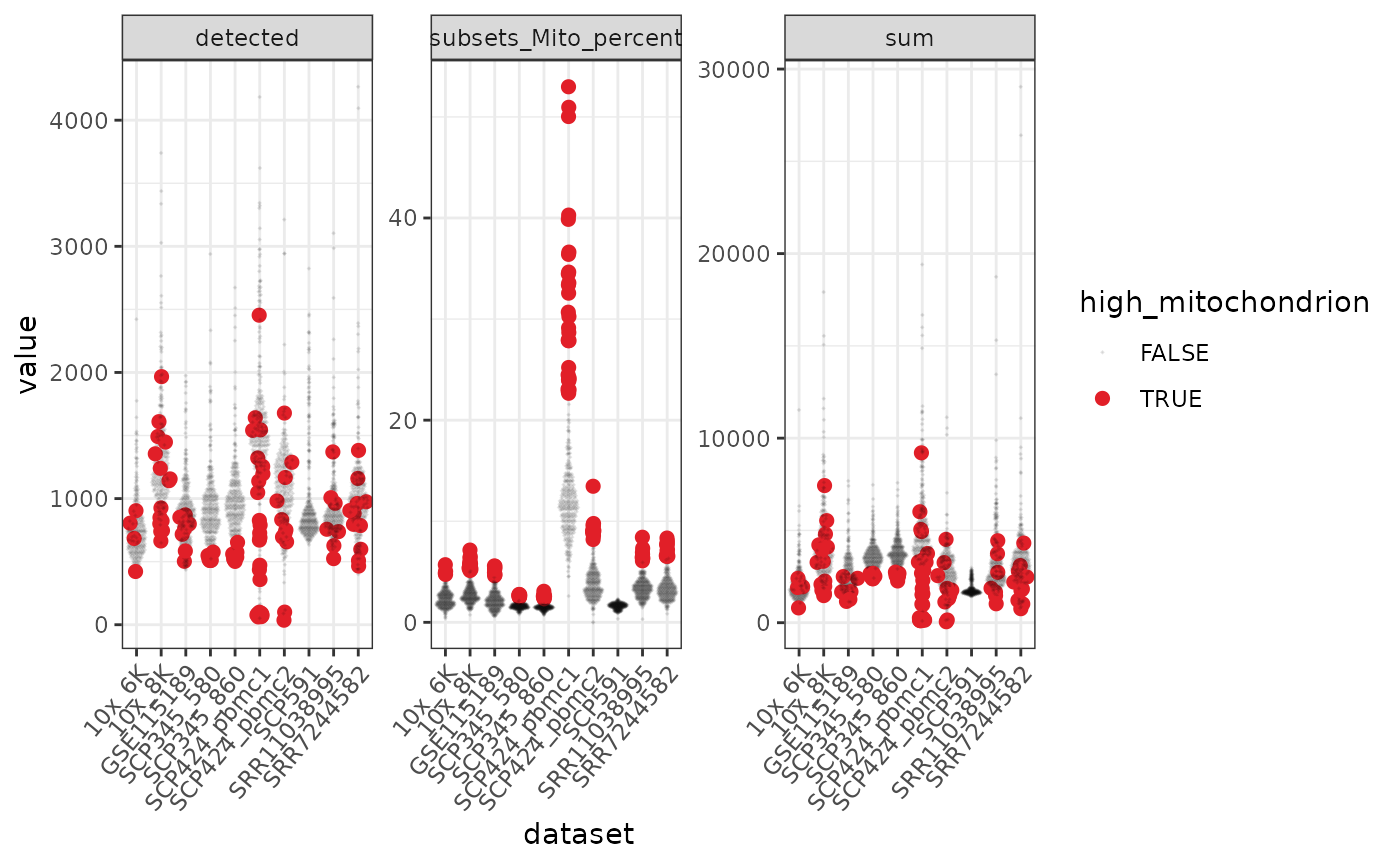
In the faceted plot, detected is number of genes in each of the 10 datasets, sum is total counts.
We filter out cells with high mitochondrial content.
pbmc_tidy <- pbmc_tidy %>% filter(!high_mitochondrion)Scaling and Integrating
We need to integrate the different datasets to adjust for technical variability between them. For integration we have chosen 10x_8K (dataset number 3) as reference because it is relatively high quality.
Identify clusters
We proceed with cluster identification with scran FindNeighbors constructs a Shared Nearest Neighbor (SNN) Graph for a given dataset. The k-nearest neighbours of each cell are first determined. FindClusters identifies clusters of cells by a shared nearest neighbour (SNN).
# Assign clusters to the 'colLabels'
# of the SingleCellExperiment object
colLabels(pbmc_tidy) <- # from SingleCellExperiment
  pbmc_tidy %>%
  buildSNNGraph(use.dimred="corrected") %>% # from scran - shared nearest neighbour
  cluster_walktrap() %$% # from igraph
  membership %>%
  as.factor()

# Reorder columns
pbmc_tidy %>% select(label, everything())
#> # A tibble abstraction: 2,899 x 8
#>    cell       label batch corrected1 corrected2 corrected3 corrected4 corrected5
#>    <chr>      <fct> <int>      <dbl>      <dbl>      <dbl>      <dbl>      <dbl>
#>  1 CCAGTCACA… 3         1   -0.0644     -0.334     -0.0725     0.0560   -0.0739
#>  2 ATGAGCACA… 6         1   -0.178       0.0167    -0.122      0.122     0.0233
#>  3 TATGAATGG… 7         1   -0.0604     -0.0357     0.127      0.293     0.0128
#>  4 CATATAGAC… 12        1   -0.0759     -0.282     -0.121      0.0545   -0.00287
#>  5 GAGGCAGAC… 2         1   -0.0758     -0.0424     0.0977     0.259     0.0248
#>  6 AGCTGCCTT… 4         1   -0.117      -0.0242    -0.0729     0.159     0.0170
#>  7 TGATTAGAT… 1         1   -0.146      -0.0752    -0.143      0.0488    0.0915
#>  8 ACGAAGCTC… 1         1   -0.119      -0.108     -0.127      0.0505    0.0624
#>  9 CGGCATCTT… 3         1   -0.00948    -0.407     -0.0466     0.0803   -0.0522
#> 10 ATAGCGTGC… 3         1   -0.0561     -0.367     -0.105      0.0589   -0.0610
#> # … with 2,889 more rows
Now we can interrogate the object as if it was a regular tibble data frame.
pbmc_tidy %>%
  count(label)
#> tidySingleCellExperiment says: A data frame is returned for independent data analysis.
#> # A tibble: 12 x 2
#>    label     n
#>    <fct> <int>
#>  1 1       367
#>  2 2       436
#>  3 3       339
#>  4 4       472
#>  5 5        21
#>  6 6       548
#>  7 7       258
#>  8 8        74
#>  9 9        41
#> 10 10      303
#> 11 11       14
#> 12 12       26
Reduce dimensions
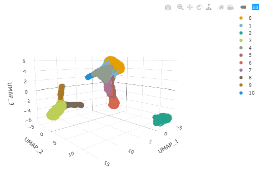
Besides PCA which is a linear dimensionality reduction, we can apply neighbour aware methods such as UMAP, to better define locally similar cells. We can calculate the first 3 UMAP dimensions using the scater framework.
# Calculate UMAP with scater
pbmc_tidy <-
  pbmc_tidy %>%
  runUMAP(ncomponents = 3, dimred="corrected") # from scater
And we can plot the clusters as a 3D plot using plotly. This time we are colouring by estimated cluster labels to visually check the cluster labels.
pbmc_tidy %>%
  plot_ly(
    x = ~`UMAP1`,
    y = ~`UMAP2`,
    z = ~`UMAP3`,
    colors = friendly_cols[1:10],
    color = ~label,
    size=0.5
  )
Cell type classification
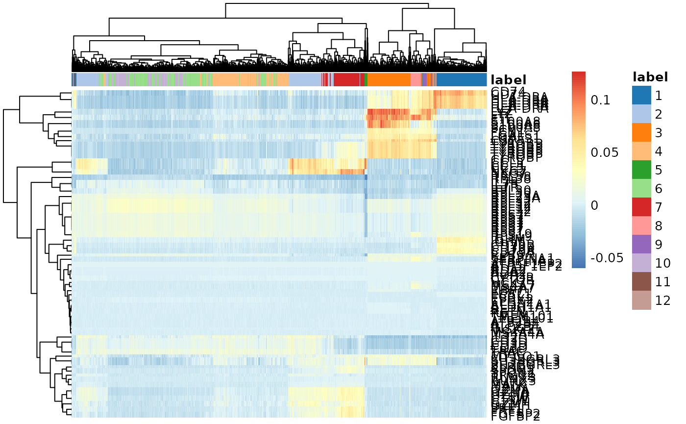
Manual cell type classification
We can identify cluster markers (genes) using scran As example, we are selecting the top 10 for each cluster. The function DoHeatmap builds an heatmap of those gene markers across cells.
# Identify top 10 markers per cluster
marker_genes <-
    pbmc_tidy %>%
    findMarkers(groups=pbmc_tidy$label, assay.type = "reconstructed") %>%  # scran
    as.list() %>%
    map(~ head(.x, 10) %>%  rownames()) %>%
    unlist()

# Plot heatmap
pbmc_tidy %>%
  plotHeatmap(                                  # from scater
    features=marker_genes,
    columns=order(pbmc_tidy$label),
    colour_columns_by=c("label"),
    exprs_values  = "reconstructed"
) 
Automatic cell type classification
We can infer cell type identities (e.g. T cell) using SingleR (Aran et al. 2019) and manipulate the output using tidyverse. SingleR accepts any log-normalised transcript abundance matrix
# Reference cell types
blueprint <- BlueprintEncodeData()
#> using temporary cache /tmp/RtmpWB3uhg/BiocFileCache
#> snapshotDate(): 2020-10-02
#> see ?celldex and browseVignettes('celldex') for documentation
#> downloading 1 resources
#> retrieving 1 resource
#> loading from cache
#> see ?celldex and browseVignettes('celldex') for documentation
#> downloading 1 resources
#> retrieving 1 resource
#> loading from cache

cell_type <-

  # extracting counts from SingleCellExperiment object
  assays(pbmc_tidy)$reconstructed%>%

    # SingleR
  SingleR(
    ref = blueprint,
    labels = blueprint$label.main,
    clusters = pbmc_tidy %>% pull(label)
  ) %>%

  # Formatting results
  as.data.frame() %>%
  as_tibble(rownames = "label") %>%
  select(label, first.labels)

cell_type
#> # A tibble: 12 x 2
#>    label first.labels
#>    <chr> <chr>
#>  1 1     B-cells
#>  2 2     NK cells
#>  3 3     Monocytes
#>  4 4     Fibroblasts
#>  5 5     Smooth muscle
#>  6 6     Skeletal muscle
#>  7 7     NK cells
#>  8 8     Neutrophils
#>  9 9     Macrophages
#> 10 10    Skeletal muscle
#> 11 11    B-cells
#> 12 12    Monocytes
We join the cluster label dataframe to our tidySingleCellExperiment tibble.
# Join cell type info
pbmc_tidy <-
  pbmc_tidy %>%
  left_join(cell_type, by = "label")

# Reorder columns
pbmc_tidy %>% select(cell, first.labels, everything())
#> # A tibble abstraction: 2,899 x 12
#>    cell  first.labels batch label corrected1 corrected2 corrected3 corrected4
#>    <chr> <chr>        <int> <chr>      <dbl>      <dbl>      <dbl>      <dbl>
#>  1 CCAG… Monocytes        1 3       -0.0644     -0.334     -0.0725     0.0560
#>  2 ATGA… Skeletal mu…     1 6       -0.178       0.0167    -0.122      0.122
#>  3 TATG… NK cells         1 7       -0.0604     -0.0357     0.127      0.293
#>  4 CATA… Monocytes        1 12      -0.0759     -0.282     -0.121      0.0545
#>  5 GAGG… NK cells         1 2       -0.0758     -0.0424     0.0977     0.259
#>  6 AGCT… Fibroblasts      1 4       -0.117      -0.0242    -0.0729     0.159
#>  7 TGAT… B-cells          1 1       -0.146      -0.0752    -0.143      0.0488
#>  8 ACGA… B-cells          1 1       -0.119      -0.108     -0.127      0.0505
#>  9 CGGC… Monocytes        1 3       -0.00948    -0.407     -0.0466     0.0803
#> 10 ATAG… Monocytes        1 3       -0.0561     -0.367     -0.105      0.0589
#> # … with 2,889 more rows, and 4 more variables: corrected5 <dbl>, UMAP1 <dbl>,
#> #   UMAP2 <dbl>, UMAP3 <dbl>
We can easily summarise the results. For example, we can see how cell type classification overlaps with cluster classification.
pbmc_tidy %>% count(label, first.labels)
#> tidySingleCellExperiment says: A data frame is returned for independent data analysis.
#> # A tibble: 12 x 3
#>    label first.labels        n
#>    <chr> <chr>           <int>
#>  1 1     B-cells           367
#>  2 10    Skeletal muscle   303
#>  3 11    B-cells            14
#>  4 12    Monocytes          26
#>  5 2     NK cells          436
#>  6 3     Monocytes         339
#>  7 4     Fibroblasts       472
#>  8 5     Smooth muscle      21
#>  9 6     Skeletal muscle   548
#> 10 7     NK cells          258
#> 11 8     Neutrophils        74
#> 12 9     Macrophages        41
Pseudobulk analyses
It is sometime useful to aggregate cell-wise transcript abundance into pseudobulk samples. It is possible to explore data and perform hypothesis testing with tools and data-source that we are more familiar with. For example, we can use edgeR in tidybulk to perform differential expression testing. For more details on pseudobulk analysis see here.
Data exploration using pseudobulk samples
To do this, we will load a helper function called aggregate_cells from GitHub Gist and use it to create a group for each sample.
# Load aggregate function
devtools::source_gist("889e4089a0e5ca2649d3c9164e3b542e")

# Aggregate
pbmc_bulk =
  tidy(pbmc) %>%
  aggregate_cells(file)

pbmc_bulk
#> # A tibble: 1,039,160 x 5
#>    file                transcript  abundance_counts abundance_logcou… orig.ident
#>    <chr>               <chr>                  <dbl>             <dbl> <chr>
#>  1 ../data/GSE115189_… DDX11L1                    0                 0 SeuratPro…
#>  2 ../data/GSE115189_… WASH7P                     0                 0 SeuratPro…
#>  3 ../data/GSE115189_… MIR6859-1                  0                 0 SeuratPro…
#>  4 ../data/GSE115189_… MIR1302-2HG                0                 0 SeuratPro…
#>  5 ../data/GSE115189_… MIR1302-2                  0                 0 SeuratPro…
#>  6 ../data/GSE115189_… FAM138A                    0                 0 SeuratPro…
#>  7 ../data/GSE115189_… OR4G4P                     0                 0 SeuratPro…
#>  8 ../data/GSE115189_… OR4G11P                    0                 0 SeuratPro…
#>  9 ../data/GSE115189_… OR4F5                      0                 0 SeuratPro…
#> 10 ../data/GSE115189_… CICP27                     0                 0 SeuratPro…
#> # … with 1,039,150 more rows
pbmc_bulk %>%

  # Tidybulk operations
  tidybulk(file, transcript, abundance_counts) %>%
  tidybulk::identify_abundant() %>%
  tidybulk::scale_abundance()
#> No group or design set. Assuming all samples belong to one group.
#> # A tibble: 1,039,160 x 9
#>    file  transcript abundance_counts abundance_logco… orig.ident .abundant   TMM
#>    <chr> <chr>                 <dbl>            <dbl> <chr>      <lgl>     <dbl>
#>  1 ../d… DDX11L1                   0                0 SeuratPro… FALSE     0.785
#>  2 ../d… WASH7P                    0                0 SeuratPro… FALSE     0.785
#>  3 ../d… MIR6859-1                 0                0 SeuratPro… FALSE     0.785
#>  4 ../d… MIR1302-2…                0                0 SeuratPro… FALSE     0.785
#>  5 ../d… MIR1302-2                 0                0 SeuratPro… FALSE     0.785
#>  6 ../d… FAM138A                   0                0 SeuratPro… FALSE     0.785
#>  7 ../d… OR4G4P                    0                0 SeuratPro… FALSE     0.785
#>  8 ../d… OR4G11P                   0                0 SeuratPro… FALSE     0.785
#>  9 ../d… OR4F5                     0                0 SeuratPro… FALSE     0.785
#> 10 ../d… CICP27                    0                0 SeuratPro… FALSE     0.785
#> # … with 1,039,150 more rows, and 2 more variables: multiplier <dbl>,
#> #   abundance_counts_scaled <dbl>
Key Points
- Some basic steps of a single-cell RNA sequencing analysis are dimensionality reduction, cluster identification and cell type classification
-
tidySingleCellExperimentis an invisible layer that operates on aSingleCellExperimentobject and enables us to visualise and manipulate data as if it were a tidy data frame. -
tidySingleCellExperimentobject is aSingleCellExperiment objectso it can be used with anySingleCellExperimentcompatible method -
tidySingleCellExperimentis an invisible layer that operates on aSingleCellExperimentobject and enables us to visualise and manipulate data as if it were a tidy data frame. -
tidySingleCellExperimentobject is aSingleCellExperiment objectso it can be used with anySingleCellExperimentcompatible method
Contributing
If you want to suggest improvements for this workshop or ask questions, you can do so as described here.
Reproducibility
Record package and version information with sessionInfo
sessionInfo()
#> R version 4.0.3 (2020-10-10)
#> Platform: x86_64-pc-linux-gnu (64-bit)
#> Running under: Ubuntu 20.04 LTS
#>
#> Matrix products: default
#> BLAS/LAPACK: /usr/lib/x86_64-linux-gnu/openblas-pthread/libopenblasp-r0.3.8.so
#>
#> locale:
#>  [1] LC_CTYPE=en_US.UTF-8       LC_NUMERIC=C
#>  [3] LC_TIME=en_US.UTF-8        LC_COLLATE=en_US.UTF-8
#>  [5] LC_MONETARY=en_US.UTF-8    LC_MESSAGES=C
#>  [7] LC_PAPER=en_US.UTF-8       LC_NAME=C
#>  [9] LC_ADDRESS=C               LC_TELEPHONE=C
#> [11] LC_MEASUREMENT=en_US.UTF-8 LC_IDENTIFICATION=C
#>
#> attached base packages:
#> [1] parallel  stats4    stats     graphics  grDevices utils     datasets
#> [8] methods   base
#>
#> other attached packages:
#>  [1] tidySingleCellExperiment_1.0.0
#>  [2] ggbeeswarm_0.6.0
#>  [3] celldex_1.0.0
#>  [4] EnsDb.Hsapiens.v86_2.99.0
#>  [5] ensembldb_2.14.0
#>  [6] AnnotationFilter_1.14.0
#>  [7] GenomicFeatures_1.42.1
#>  [8] AnnotationDbi_1.52.0
#>  [9] scuttle_1.0.3
#> [10] SingleR_1.4.0
#> [11] batchelor_1.6.2
#> [12] igraph_1.2.6
#> [13] scran_1.18.2
#> [14] scater_1.18.3
#> [15] SingleCellExperiment_1.12.0
#> [16] purrr_0.3.4
#> [17] bioceurope2020tidytranscriptomics_0.7.3
#> [18] tidySummarizedExperiment_1.0.0
#> [19] tidybulk_1.2.0
#> [20] tidyHeatmap_1.1.5
#> [21] GGally_2.0.0
#> [22] ggrepel_0.8.2
#> [23] plotly_4.9.2.1
#> [24] ggplot2_3.3.2
#> [25] stringr_1.4.0
#> [26] readr_1.4.0
#> [27] tidyr_1.1.2
#> [28] dplyr_1.0.2
#> [29] tibble_3.0.4
#> [30] airway_1.10.0
#> [31] SummarizedExperiment_1.20.0
#> [32] Biobase_2.50.0
#> [33] GenomicRanges_1.42.0
#> [34] GenomeInfoDb_1.26.2
#> [35] IRanges_2.24.1
#> [36] S4Vectors_0.28.1
#> [37] BiocGenerics_0.36.0
#> [38] MatrixGenerics_1.2.0
#> [39] matrixStats_0.57.0
#>
#> loaded via a namespace (and not attached):
#>   [1] utf8_1.1.4                    tidyselect_1.1.0
#>   [3] RSQLite_2.2.1                 htmlwidgets_1.5.3
#>   [5] grid_4.0.3                    BiocParallel_1.24.1
#>   [7] devtools_2.3.2                munsell_0.5.0
#>   [9] ragg_0.4.0                    preprocessCore_1.52.0
#>  [11] statmod_1.4.35                withr_2.3.0
#>  [13] colorspace_2.0-0              knitr_1.30
#>  [15] labeling_0.4.2                GenomeInfoDbData_1.2.4
#>  [17] bit64_4.0.5                   farver_2.0.3
#>  [19] pheatmap_1.0.12               rprojroot_2.0.2
#>  [21] vctrs_0.3.5                   generics_0.1.0
#>  [23] xfun_0.19                     dittoSeq_1.2.2
#>  [25] BiocFileCache_1.14.0          R6_2.5.0
#>  [27] clue_0.3-58                   rsvd_1.0.3
#>  [29] locfit_1.5-9.4                bitops_1.0-6
#>  [31] reshape_0.8.8                 DelayedArray_0.16.0
#>  [33] assertthat_0.2.1              promises_1.1.1
#>  [35] scales_1.1.1                  beeswarm_0.2.3
#>  [37] gtable_0.3.0                  beachmat_2.6.3
#>  [39] Cairo_1.5-12.2                processx_3.4.5
#>  [41] rlang_0.4.9                   genefilter_1.72.0
#>  [43] systemfonts_0.3.2             GlobalOptions_0.1.2
#>  [45] splines_4.0.3                 rtracklayer_1.50.0
#>  [47] lazyeval_0.2.2                BiocManager_1.30.10
#>  [49] yaml_2.2.1                    httpuv_1.5.4
#>  [51] usethis_2.0.0                 tools_4.0.3
#>  [53] ellipsis_0.3.1                RColorBrewer_1.1-2
#>  [55] sessioninfo_1.1.1             ggridges_0.5.2
#>  [57] Rcpp_1.0.5                    plyr_1.8.6
#>  [59] sparseMatrixStats_1.2.0       progress_1.2.2
#>  [61] zlibbioc_1.36.0               RCurl_1.98-1.2
#>  [63] ps_1.5.0                      prettyunits_1.1.1
#>  [65] openssl_1.4.3                 GetoptLong_1.0.4
#>  [67] viridis_0.5.1                 cowplot_1.1.0
#>  [69] cluster_2.1.0                 fs_1.5.0
#>  [71] magrittr_2.0.1                RSpectra_0.16-0
#>  [73] data.table_1.13.4             ResidualMatrix_1.0.0
#>  [75] circlize_0.4.11               ProtGenerics_1.22.0
#>  [77] pkgload_1.1.0                 mime_0.9
#>  [79] hms_0.5.3                     evaluate_0.14
#>  [81] xtable_1.8-4                  XML_3.99-0.5
#>  [83] gridExtra_2.3                 shape_1.4.5
#>  [85] testthat_3.0.0                compiler_4.0.3
#>  [87] biomaRt_2.46.0                crayon_1.3.4
#>  [89] htmltools_0.5.0               later_1.1.0.1
#>  [91] geneplotter_1.68.0            DBI_1.1.0
#>  [93] ExperimentHub_1.16.0          dbplyr_2.0.0
#>  [95] ComplexHeatmap_2.6.2          rappdirs_0.3.1
#>  [97] Matrix_1.2-18                 cli_2.2.0
#>  [99] pkgconfig_2.0.3               pkgdown_1.6.1
#> [101] GenomicAlignments_1.26.0      xml2_1.3.2
#> [103] annotate_1.68.0               vipor_0.4.5
#> [105] dqrng_0.2.1                   XVector_0.30.0
#> [107] callr_3.5.1                   digest_0.6.27
#> [109] Biostrings_2.58.0             rmarkdown_2.6
#> [111] uwot_0.1.9                    edgeR_3.32.0
#> [113] DelayedMatrixStats_1.12.1     curl_4.3
#> [115] shiny_1.5.0                   Rsamtools_2.6.0
#> [117] rjson_0.2.20                  lifecycle_0.2.0
#> [119] jsonlite_1.7.2                BiocNeighbors_1.8.2
#> [121] desc_1.2.0                    viridisLite_0.3.0
#> [123] askpass_1.1                   limma_3.46.0
#> [125] fansi_0.4.1                   pillar_1.4.7
#> [127] lattice_0.20-41               pkgbuild_1.1.0
#> [129] fastmap_1.0.1                 httr_1.4.2
#> [131] survival_3.2-7                remotes_2.2.0
#> [133] interactiveDisplayBase_1.28.0 glue_1.4.2
#> [135] FNN_1.1.3                     png_0.1-7
#> [137] bluster_1.0.0                 BiocVersion_3.12.0
#> [139] bit_4.0.4                     class_7.3-17
#> [141] stringi_1.5.3                 blob_1.2.1
#> [143] textshaping_0.2.1             DESeq2_1.30.0
#> [145] org.Hs.eg.db_3.12.0           BiocSingular_1.6.0
#> [147] AnnotationHub_2.22.0          memoise_1.1.0
#> [149] irlba_2.3.3                   e1071_1.7-4
References
Abbas, Alexander R, Kristen Wolslegel, Dhaya Seshasayee, Zora Modrusan, and Hilary F Clark. 2009. “Deconvolution of Blood Microarray Data Identifies Cellular Activation Patterns in Systemic Lupus Erythematosus.” PloS One 4 (7): e6098.
Aran, Dvir, Agnieszka P Looney, Leqian Liu, Esther Wu, Valerie Fong, Austin Hsu, Suzanna Chak, et al. 2019. “Reference-Based Analysis of Lung Single-Cell Sequencing Reveals a Transitional Profibrotic Macrophage.” Nature Immunology 20 (2): 163–72.
Cai, Yi, Youchao Dai, Yejun Wang, Qianqing Yang, Jiubiao Guo, Cailing Wei, Weixin Chen, et al. 2020. “Single-Cell Transcriptomics of Blood Reveals a Natural Killer Cell Subset Depletion in Tuberculosis.” EBioMedicine 53 (March): 102686. https://doi.org/10.1016/j.ebiom.2020.102686.
Chen, Yunshun, Aaron TL Lun, and Gordon K Smyth. 2016. “From Reads to Genes to Pathways: Differential Expression Analysis of Rna-Seq Experiments Using Rsubread and the edgeR Quasi-Likelihood Pipeline.” F1000Research 5.
Ding, Jiarui, Xian Adiconis, Sean K. Simmons, Monika S. Kowalczyk, Cynthia C. Hession, Nemanja D. Marjanovic, Travis K. Hughes, et al. 2020. “Systematic Comparison of Single-Cell and Single-Nucleus RNA-Sequencing Methods.” Nature Biotechnology 38 (6): 737–46. https://doi.org/10.1038/s41587-020-0465-8.
Freytag, Saskia, Luyi Tian, Ingrid Lönnstedt, Milica Ng, and Melanie Bahlo. 2018. “Comparison of Clustering Tools in R for Medium-Sized 10x Genomics Single-Cell RNA-Sequencing Data.” F1000Research 7 (December): 1297. https://doi.org/10.12688/f1000research.15809.2.
Himes, Blanca E, Xiaofeng Jiang, Peter Wagner, Ruoxi Hu, Qiyu Wang, Barbara Klanderman, Reid M Whitaker, et al. 2014. “RNA-Seq Transcriptome Profiling Identifies Crispld2 as a Glucocorticoid Responsive Gene That Modulates Cytokine Function in Airway Smooth Muscle Cells.” PloS One 9 (6): e99625.
Karagiannis, Tanya T., John P. Cleary, Busra Gok, Andrew J. Henderson, Nicholas G. Martin, Masanao Yajima, Elliot C. Nelson, and Christine S. Cheng. 2020. “Single Cell Transcriptomics Reveals Opioid Usage Evokes Widespread Suppression of Antiviral Gene Program.” Nature Communications 11 (1). https://doi.org/10.1038/s41467-020-16159-y.
Law, Charity W, Monther Alhamdoosh, Shian Su, Xueyi Dong, Luyi Tian, Gordon K Smyth, and Matthew E Ritchie. 2016. “RNA-Seq Analysis Is Easy as 1-2-3 with Limma, Glimma and edgeR.” F1000Research 5.
Law, Charity W, Yunshun Chen, Wei Shi, and Gordon K Smyth. 2014. “Voom: Precision Weights Unlock Linear Model Analysis Tools for Rna-Seq Read Counts.” Genome Biology 15 (2): R29.
Love, Michael I, Wolfgang Huber, and Simon Anders. 2014. “Moderated Estimation of Fold Change and Dispersion for Rna-Seq Data with Deseq2.” Genome Biology 15 (12): 550.
Mangiola, Stefano, and Anthony T Papenfuss. 2020. “TidyHeatmap: An R Package for Modular Heatmap Production Based on Tidy Principles.” Journal of Open Source Software 5 (52): 2472.
McCarthy, Davis J, Yunshun Chen, and Gordon K Smyth. 2012. “Differential Expression Analysis of Multifactor Rna-Seq Experiments with Respect to Biological Variation.” Nucleic Acids Research 40 (10): 4288–97.
Newman, Aaron M, Chih Long Liu, Michael R Green, Andrew J Gentles, Weiguo Feng, Yue Xu, Chuong D Hoang, Maximilian Diehn, and Ash A Alizadeh. 2015. “Robust Enumeration of Cell Subsets from Tissue Expression Profiles.” Nature Methods 12 (5): 453–57.
Racle, Julien, Kaat de Jonge, Petra Baumgaertner, Daniel E Speiser, and David Gfeller. 2017. “Simultaneous Enumeration of Cancer and Immune Cell Types from Bulk Tumor Gene Expression Data.” Elife 6: e26476.
Robinson, Mark D, and Alicia Oshlack. 2010. “A Scaling Normalization Method for Differential Expression Analysis of Rna-Seq Data.” Genome Biology 11 (3): 1–9.
Wickham, Hadley, Mara Averick, Jennifer Bryan, Winston Chang, Lucy D’Agostino McGowan, Romain François, Garrett Grolemund, et al. 2019. “Welcome to the Tidyverse.” Journal of Open Source Software 4 (43): 1686.
Wickham, Hadley, and others. 2014. “Tidy Data.” Journal of Statistical Software 59 (10): 1–23.