tidybulk - part of tidyTranscriptomics

Brings transcriptomics to the tidyverse!

The code is released under the version 3 of the GNU General Public License.

website: stemangiola.github.io/tidybulk/

Please have a look also to

• tidySummarizedExperiment for bulk data tidy representation
• tidySingleCellExperiment for single-cell data tidy representation
• tidyseurat for single-cell data tidy representation
• tidyHeatmap for heatmaps produced with tidy principles analysis and manipulation
• nanny for tidy high-level data analysis and manipulation
• tidygate for adding custom gate information to your tibble

Functions/utilities available

Function	Description
aggregate_duplicates	Aggregate abundance and annotation of duplicated transcripts in a robust way
identify_abundant keep_abundant	identify or keep the abundant genes
keep_variable	Filter for top variable features
scale_abundance	Scale (normalise) abundance for RNA sequencing depth
reduce_dimensions	Perform dimensionality reduction (PCA, MDS, tSNE, UMAP)
cluster_elements	Labels elements with cluster identity (kmeans, SNN)
remove_redundancy	Filter out elements with highly correlated features
adjust_abundance	Remove known unwanted variation (Combat)
test_differential_abundance	Differential transcript abundance testing (DESeq2, edgeR, voom)
deconvolve_cellularity	Estimated tissue composition (Cibersort, llsr, epic, xCell, mcp_counter, quantiseq
test_differential_cellularity	Differential cell-type abundance testing
test_stratification_cellularity	Estimate Kaplan-Meier survival differences
test_gene_enrichment	Gene enrichment analyses (EGSEA)
test_gene_overrepresentation	Gene enrichment on list of transcript names (no rank)
test_gene_rank	Gene enrichment on list of transcript (GSEA)
impute_missing_abundance	Impute abundance for missing data points using sample groupings

Utilities	Description
get_bibliography	Get the bibliography of your workflow
tidybulk	add tidybulk attributes to a tibble object
tidybulk_SAM_BAM	Convert SAM BAM files into tidybulk tibble
pivot_sample	Select sample-wise columns/information
pivot_transcript	Select transcript-wise columns/information
rotate_dimensions	Rotate two dimensions of a degree
ensembl_to_symbol	Add gene symbol from ensembl IDs
symbol_to_entrez	Add entrez ID from gene symbol
describe_transcript	Add gene description from gene symbol

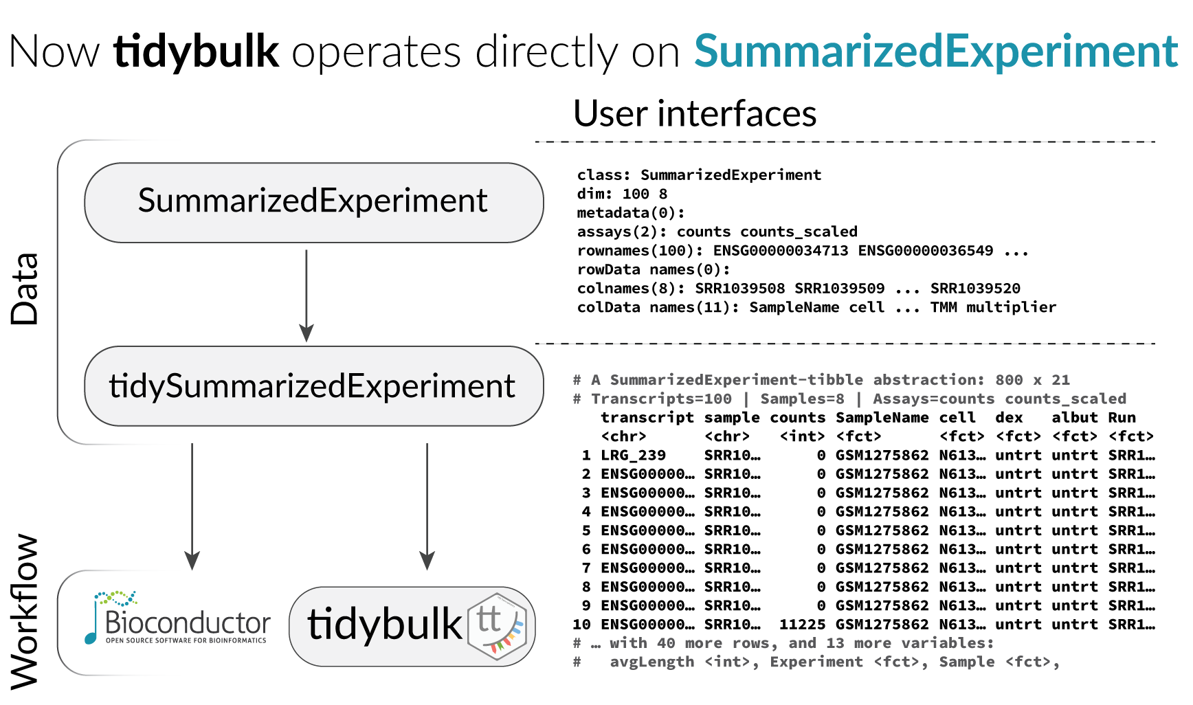
All functions are directly compatibble with SummarizedExperiment object.

Installation

From Bioconductor

BiocManager::install("tidybulk")

From Github

devtools::install_github("stemangiola/tidybulk")

Data

We will use a SummarizedExperiment object

counts_SE

## # A SummarizedExperiment-tibble abstraction: 408,624 × 48
## # [90mFeatures=8513 | Samples=48 | Assays=count[0m
##    .feature .sample    count Cell.type time  condition batch factor_of_interest
##    <chr>    <chr>      <dbl> <fct>     <fct> <lgl>     <fct> <lgl>             
##  1 A1BG     SRR1740034   153 b_cell    0 d   TRUE      0     TRUE              
##  2 A1BG-AS1 SRR1740034    83 b_cell    0 d   TRUE      0     TRUE              
##  3 AAAS     SRR1740034   868 b_cell    0 d   TRUE      0     TRUE              
##  4 AACS     SRR1740034   222 b_cell    0 d   TRUE      0     TRUE              
##  5 AAGAB    SRR1740034   590 b_cell    0 d   TRUE      0     TRUE              
##  6 AAMDC    SRR1740034    48 b_cell    0 d   TRUE      0     TRUE              
##  7 AAMP     SRR1740034  1257 b_cell    0 d   TRUE      0     TRUE              
##  8 AANAT    SRR1740034   284 b_cell    0 d   TRUE      0     TRUE              
##  9 AAR2     SRR1740034   379 b_cell    0 d   TRUE      0     TRUE              
## 10 AARS2    SRR1740034   685 b_cell    0 d   TRUE      0     TRUE              
## # … with 40 more rows
## # ℹ Use `print(n = ...)` to see more rows

Loading tidySummarizedExperiment will automatically abstract this object as tibble, so we can display it and manipulate it with tidy tools. Although it looks different, and more tools (tidyverse) are available to us, this object is in fact a SummarizedExperiment object.

class(counts_SE)

## [1] "SummarizedExperiment"
## attr(,"package")
## [1] "SummarizedExperiment"

Get the bibliography of your workflow

First of all, you can cite all articles utilised within your workflow automatically from any tidybulk tibble

counts_SE %>%   get_bibliography()

Aggregate duplicated transcripts

tidybulk provide the aggregate_duplicates function to aggregate duplicated transcripts (e.g., isoforms, ensembl). For example, we often have to convert ensembl symbols to gene/transcript symbol, but in doing so we have to deal with duplicates. aggregate_duplicates takes a tibble and column names (as symbols; for sample, transcript and count) as arguments and returns a tibble with transcripts with the same name aggregated. All the rest of the columns are appended, and factors and boolean are appended as characters.

TidyTranscriptomics

rowData(counts_SE)$gene_name = rownames(counts_SE)
counts_SE.aggr = counts_SE %>% aggregate_duplicates(.transcript = gene_name)

Standard procedure (comparative purpose)

temp = data.frame(
    symbol = dge_list$genes$symbol,
    dge_list$counts
)
dge_list.nr <- by(temp, temp$symbol,
    function(df)
        if(length(df[1,1])>0)
            matrixStats:::colSums(as.matrix(df[,-1]))
)
dge_list.nr <- do.call("rbind", dge_list.nr)
colnames(dge_list.nr) <- colnames(dge_list)

Scale counts

We may want to compensate for sequencing depth, scaling the transcript abundance (e.g., with TMM algorithm, Robinson and Oshlack doi.org/10.1186/gb-2010-11-3-r25). scale_abundance takes a tibble, column names (as symbols; for sample, transcript and count) and a method as arguments and returns a tibble with additional columns with scaled data as <NAME OF COUNT COLUMN>_scaled.

TidyTranscriptomics

counts_SE.norm = counts_SE.aggr %>% identify_abundant(factor_of_interest = condition) %>% scale_abundance()

Standard procedure (comparative purpose)

library(edgeR)

dgList <- DGEList(count_m=x,group=group)
keep <- filterByExpr(dgList)
dgList <- dgList[keep,,keep.lib.sizes=FALSE]
[...]
dgList <- calcNormFactors(dgList, method="TMM")
norm_counts.table <- cpm(dgList)

We can easily plot the scaled density to check the scaling outcome. On the x axis we have the log scaled counts, on the y axes we have the density, data is grouped by sample and coloured by cell type.

counts_SE.norm %>%
    ggplot(aes(count_scaled + 1, group=sample, color=`Cell.type`)) +
    geom_density() +
    scale_x_log10() +
    my_theme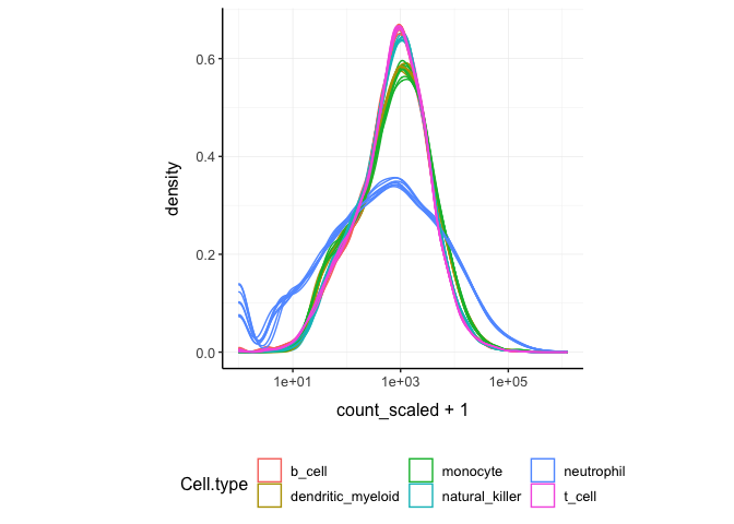

Filter variable transcripts

We may want to identify and filter variable transcripts.

TidyTranscriptomics

counts_SE.norm.variable = counts_SE.norm %>% keep_variable()

Standard procedure (comparative purpose)

library(edgeR)

x = norm_counts.table

s <- rowMeans((x-rowMeans(x))^2)
o <- order(s,decreasing=TRUE)
x <- x[o[1L:top],,drop=FALSE]

norm_counts.table = norm_counts.table[rownames(x)]

norm_counts.table$cell_type = tibble_counts[
    match(
        tibble_counts$sample,
        rownames(norm_counts.table)
    ),
    "Cell.type"
]

Reduce dimensions

We may want to reduce the dimensions of our data, for example using PCA or MDS algorithms. reduce_dimensions takes a tibble, column names (as symbols; for sample, transcript and count) and a method (e.g., MDS or PCA) as arguments and returns a tibble with additional columns for the reduced dimensions.

MDS (Robinson et al., 10.1093/bioinformatics/btp616)

TidyTranscriptomics

counts_SE.norm.MDS =
  counts_SE.norm %>%
  reduce_dimensions(method="MDS", .dims = 6)

Standard procedure (comparative purpose)

library(limma)

count_m_log = log(count_m + 1)
cmds = limma::plotMDS(ndim = .dims, plot = FALSE)

cmds = cmds %$% 
    cmdscale.out %>%
    setNames(sprintf("Dim%s", 1:6))

cmds$cell_type = tibble_counts[
    match(tibble_counts$sample, rownames(cmds)),
    "Cell.type"
]

On the x and y axes axis we have the reduced dimensions 1 to 3, data is coloured by cell type.

counts_SE.norm.MDS %>% pivot_sample()  %>% select(contains("Dim"), everything())

## # A tibble: 48 × 14
##      Dim1   Dim2   Dim3     Dim4    Dim5    Dim6 .sample   Cell.…¹ time  condi…²
##     <dbl>  <dbl>  <dbl>    <dbl>   <dbl>   <dbl> <chr>     <fct>   <fct> <lgl>  
##  1 -1.46   0.220 -1.68   0.0553   0.0658 -0.126  SRR17400… b_cell  0 d   TRUE   
##  2 -1.46   0.226 -1.71   0.0300   0.0454 -0.137  SRR17400… b_cell  1 d   TRUE   
##  3 -1.44   0.193 -1.60   0.0890   0.0503 -0.121  SRR17400… b_cell  3 d   TRUE   
##  4 -1.44   0.198 -1.67   0.0891   0.0543 -0.110  SRR17400… b_cell  7 d   TRUE   
##  5  0.243 -1.42   0.182  0.00642 -0.503  -0.131  SRR17400… dendri… 0 d   FALSE  
##  6  0.191 -1.42   0.195  0.0180  -0.457  -0.130  SRR17400… dendri… 1 d   FALSE  
##  7  0.257 -1.42   0.152  0.0130  -0.582  -0.0927 SRR17400… dendri… 3 d   FALSE  
##  8  0.162 -1.43   0.189  0.0232  -0.452  -0.109  SRR17400… dendri… 7 d   FALSE  
##  9  0.516 -1.47   0.240 -0.251    0.457  -0.119  SRR17400… monocy… 0 d   FALSE  
## 10  0.514 -1.41   0.231 -0.219    0.458  -0.131  SRR17400… monocy… 1 d   FALSE  
## # … with 38 more rows, 4 more variables: batch <fct>, factor_of_interest <lgl>,
## #   TMM <dbl>, multiplier <dbl>, and abbreviated variable names ¹​Cell.type,
## #   ²​condition
## # ℹ Use `print(n = ...)` to see more rows, and `colnames()` to see all variable names

counts_SE.norm.MDS %>%
    pivot_sample() %>%
  GGally::ggpairs(columns = 6:(6+5), ggplot2::aes(colour=`Cell.type`))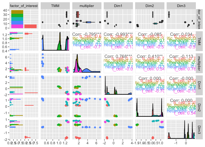

PCA

TidyTranscriptomics

counts_SE.norm.PCA =
  counts_SE.norm %>%
  reduce_dimensions(method="PCA", .dims = 6)

Standard procedure (comparative purpose)

count_m_log = log(count_m + 1)
pc = count_m_log %>% prcomp(scale = TRUE)
variance = pc$sdev^2
variance = (variance / sum(variance))[1:6]
pc$cell_type = counts[
    match(counts$sample, rownames(pc)),
    "Cell.type"
]

On the x and y axes axis we have the reduced dimensions 1 to 3, data is coloured by cell type.

counts_SE.norm.PCA %>% pivot_sample() %>% select(contains("PC"), everything())

## # A tibble: 48 × 14
##        PC1   PC2    PC3     PC4    PC5   PC6 .sample Cell.…¹ time  condi…² batch
##      <dbl> <dbl>  <dbl>   <dbl>  <dbl> <dbl> <chr>   <fct>   <fct> <lgl>   <fct>
##  1 -12.6   -2.52 -14.9  -0.424  -0.592 -1.22 SRR174… b_cell  0 d   TRUE    0    
##  2 -12.6   -2.57 -15.2  -0.140  -0.388 -1.30 SRR174… b_cell  1 d   TRUE    1    
##  3 -12.6   -2.41 -14.5  -0.714  -0.344 -1.10 SRR174… b_cell  3 d   TRUE    1    
##  4 -12.5   -2.34 -14.9  -0.816  -0.427 -1.00 SRR174… b_cell  7 d   TRUE    1    
##  5   0.189 13.0    1.66 -0.0269  4.64  -1.35 SRR174… dendri… 0 d   FALSE   0    
##  6  -0.293 12.9    1.76 -0.0727  4.21  -1.28 SRR174… dendri… 1 d   FALSE   0    
##  7   0.407 13.0    1.42 -0.0529  5.37  -1.01 SRR174… dendri… 3 d   FALSE   1    
##  8  -0.620 13.0    1.73 -0.201   4.17  -1.07 SRR174… dendri… 7 d   FALSE   0    
##  9   2.56  13.5    2.32  2.03   -4.32  -1.22 SRR174… monocy… 0 d   FALSE   1    
## 10   2.65  13.1    2.21  1.80   -4.29  -1.30 SRR174… monocy… 1 d   FALSE   1    
## # … with 38 more rows, 3 more variables: factor_of_interest <lgl>, TMM <dbl>,
## #   multiplier <dbl>, and abbreviated variable names ¹​Cell.type, ²​condition
## # ℹ Use `print(n = ...)` to see more rows, and `colnames()` to see all variable names

counts_SE.norm.PCA %>%
     pivot_sample() %>%
  GGally::ggpairs(columns = 11:13, ggplot2::aes(colour=`Cell.type`))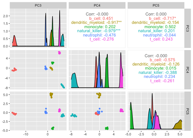

tSNE

TidyTranscriptomics

counts_SE.norm.tSNE =
    breast_tcga_mini_SE %>%
    identify_abundant() %>%
    reduce_dimensions(
        method = "tSNE",
        perplexity=10,
        pca_scale =TRUE
    )

Standard procedure (comparative purpose)

count_m_log = log(count_m + 1)

tsne = Rtsne::Rtsne(
    t(count_m_log),
    perplexity=10,
        pca_scale =TRUE
)$Y
tsne$cell_type = tibble_counts[
    match(tibble_counts$sample, rownames(tsne)),
    "Cell.type"
]

Plot

counts_SE.norm.tSNE %>%
    pivot_sample() %>%
    select(contains("tSNE"), everything()) 

## # A tibble: 251 × 4
##     tSNE1  tSNE2 .sample                      Call 
##     <dbl>  <dbl> <chr>                        <fct>
##  1  -5.25  10.2  TCGA-A1-A0SD-01A-11R-A115-07 LumA 
##  2   6.41   2.79 TCGA-A1-A0SF-01A-11R-A144-07 LumA 
##  3  -9.28   6.63 TCGA-A1-A0SG-01A-11R-A144-07 LumA 
##  4  -1.76   4.82 TCGA-A1-A0SH-01A-11R-A084-07 LumA 
##  5  -1.41  12.2  TCGA-A1-A0SI-01A-11R-A144-07 LumB 
##  6  -1.89  -3.60 TCGA-A1-A0SJ-01A-11R-A084-07 LumA 
##  7  18.5  -13.4  TCGA-A1-A0SK-01A-12R-A084-07 Basal
##  8  -4.03 -10.4  TCGA-A1-A0SM-01A-11R-A084-07 LumA 
##  9  -2.84 -10.8  TCGA-A1-A0SN-01A-11R-A144-07 LumB 
## 10 -19.3    5.03 TCGA-A1-A0SQ-01A-21R-A144-07 LumA 
## # … with 241 more rows
## # ℹ Use `print(n = ...)` to see more rows

counts_SE.norm.tSNE %>%
    pivot_sample() %>%
    ggplot(aes(x = `tSNE1`, y = `tSNE2`, color=Call)) + geom_point() + my_theme

Rotate dimensions

We may want to rotate the reduced dimensions (or any two numeric columns really) of our data, of a set angle. rotate_dimensions takes a tibble, column names (as symbols; for sample, transcript and count) and an angle as arguments and returns a tibble with additional columns for the rotated dimensions. The rotated dimensions will be added to the original data set as <NAME OF DIMENSION> rotated <ANGLE> by default, or as specified in the input arguments.

TidyTranscriptomics

counts_SE.norm.MDS.rotated =
  counts_SE.norm.MDS %>%
    rotate_dimensions(`Dim1`, `Dim2`, rotation_degrees = 45, action="get")

Standard procedure (comparative purpose)

rotation = function(m, d) {
    r = d * pi / 180
    ((bind_rows(
        c(`1` = cos(r), `2` = -sin(r)),
        c(`1` = sin(r), `2` = cos(r))
    ) %>% as_matrix) %*% m)
}
mds_r = pca %>% rotation(rotation_degrees)
mds_r$cell_type = counts[
    match(counts$sample, rownames(mds_r)),
    "Cell.type"
]

Original On the x and y axes axis we have the first two reduced dimensions, data is coloured by cell type.

counts_SE.norm.MDS.rotated %>%
    ggplot(aes(x=`Dim1`, y=`Dim2`, color=`Cell.type` )) +
  geom_point() +
  my_theme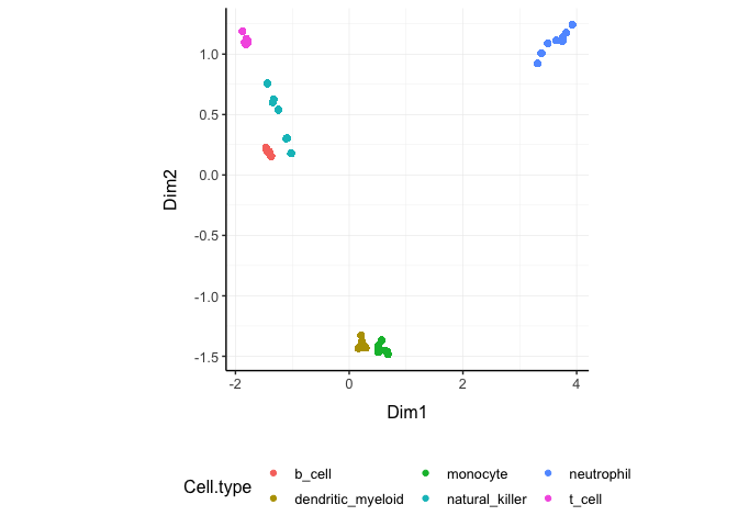

Rotated On the x and y axes axis we have the first two reduced dimensions rotated of 45 degrees, data is coloured by cell type.

counts_SE.norm.MDS.rotated %>%
    pivot_sample() %>%
    ggplot(aes(x=`Dim1_rotated_45`, y=`Dim2_rotated_45`, color=`Cell.type` )) +
  geom_point() +
  my_theme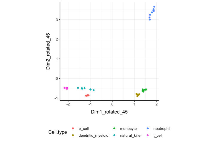

Test differential abundance

We may want to test for differential transcription between sample-wise factors of interest (e.g., with edgeR). test_differential_abundance takes a tibble, column names (as symbols; for sample, transcript and count) and a formula representing the desired linear model as arguments and returns a tibble with additional columns for the statistics from the hypothesis test (e.g., log fold change, p-value and false discovery rate).

TidyTranscriptomics

counts_SE.de =
    counts_SE %>%
    test_differential_abundance( ~ condition, action="get")
counts_SE.de

Standard procedure (comparative purpose)

library(edgeR)

dgList <- DGEList(counts=counts_m,group=group)
keep <- filterByExpr(dgList)
dgList <- dgList[keep,,keep.lib.sizes=FALSE]
dgList <- calcNormFactors(dgList)
design <- model.matrix(~group)
dgList <- estimateDisp(dgList,design)
fit <- glmQLFit(dgList,design)
qlf <- glmQLFTest(fit,coef=2)
topTags(qlf, n=Inf)

The functon test_differential_abundance operated with contrasts too. The constrasts hve the name of the design matrix (generally )

counts_SE.de =
    counts_SE %>%
    identify_abundant(factor_of_interest = condition) %>%
    test_differential_abundance(
        ~ 0 + condition,                  
        .contrasts = c( "conditionTRUE - conditionFALSE"),
        action="get"
    )

Adjust counts

We may want to adjust counts for (known) unwanted variation. adjust_abundance takes as arguments a tibble, column names (as symbols; for sample, transcript and count) and a formula representing the desired linear model where the first covariate is the factor of interest and the second covariate is the unwanted variation, and returns a tibble with additional columns for the adjusted counts as <COUNT COLUMN>_adjusted. At the moment just an unwanted covariated is allowed at a time.

TidyTranscriptomics

counts_SE.norm.adj =
    counts_SE.norm %>% adjust_abundance(    ~ factor_of_interest + batch)

Standard procedure (comparative purpose)

library(sva)

count_m_log = log(count_m + 1)

design =
        model.matrix(
            object = ~ factor_of_interest + batch,
            data = annotation
        )

count_m_log.sva =
    ComBat(
            batch = design[,2],
            mod = design,
            ...
        )

count_m_log.sva = ceiling(exp(count_m_log.sva) -1)
count_m_log.sva$cell_type = counts[
    match(counts$sample, rownames(count_m_log.sva)),
    "Cell.type"
]

Deconvolve Cell type composition

We may want to infer the cell type composition of our samples (with the algorithm Cibersort; Newman et al., 10.1038/nmeth.3337). deconvolve_cellularity takes as arguments a tibble, column names (as symbols; for sample, transcript and count) and returns a tibble with additional columns for the adjusted cell type proportions.

TidyTranscriptomics

counts_SE.cibersort =
    counts_SE %>%
    deconvolve_cellularity(action="get", cores=1, prefix = "cibersort__") 

## 
## The downloaded binary packages are in
##  /var/folders/zn/m_qvr9zd7tq0wdtsbq255f8xypj_zg/T//RtmpIi5KN6/downloaded_packages

Standard procedure (comparative purpose)

source(‘CIBERSORT.R’)
count_m %>% write.table("mixture_file.txt")
results <- CIBERSORT(
    "sig_matrix_file.txt",
    "mixture_file.txt",
    perm=100, QN=TRUE
)
results$cell_type = tibble_counts[
    match(tibble_counts$sample, rownames(results)),
    "Cell.type"
]

With the new annotated data frame, we can plot the distributions of cell types across samples, and compare them with the nominal cell type labels to check for the purity of isolation. On the x axis we have the cell types inferred by Cibersort, on the y axis we have the inferred proportions. The data is facetted and coloured by nominal cell types (annotation given by the researcher after FACS sorting).

counts_SE.cibersort %>%
    pivot_longer(
        names_to= "Cell_type_inferred", 
        values_to = "proportion", 
        names_prefix ="cibersort__", 
        cols=contains("cibersort__")
    ) %>%
  ggplot(aes(x=`Cell_type_inferred`, y=proportion, fill=`Cell.type`)) +
  geom_boxplot() +
  facet_wrap(~`Cell.type`) +
  my_theme +
  theme(axis.text.x = element_text(angle = 90, hjust = 1, vjust = 0.5), aspect.ratio=1/5)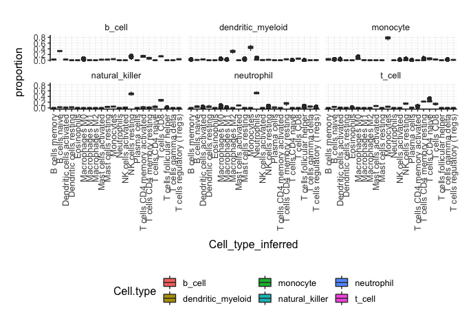

Test differential cell-type abundance

We can also perform a statistical test on the differential cell-type abundance across conditions

    counts_SE %>%
    test_differential_cellularity(. ~ condition )

## 
## The downloaded binary packages are in
##  /var/folders/zn/m_qvr9zd7tq0wdtsbq255f8xypj_zg/T//RtmpIi5KN6/downloaded_packages

## # A tibble: 22 × 7
##    .cell_type                  cell_t…¹ estim…² estim…³ std.e…⁴ stati…⁵ p.valu…⁶
##    <chr>                       <list>     <dbl>   <dbl>   <dbl>   <dbl>    <dbl>
##  1 cibersort.B.cells.naive     <tibble>   -2.94   2.25    0.367   6.13  8.77e-10
##  2 cibersort.B.cells.memory    <tibble>   -4.86   1.48    0.436   3.40  6.77e- 4
##  3 cibersort.Plasma.cells      <tibble>   -5.33  -0.487   0.507  -0.960 3.37e- 1
##  4 cibersort.T.cells.CD8       <tibble>   -2.33   0.924   0.475   1.94  5.18e- 2
##  5 cibersort.T.cells.CD4.naive <tibble>   -2.83  -0.620   0.531  -1.17  2.43e- 1
##  6 cibersort.T.cells.CD4.memo… <tibble>   -2.46   0.190   0.500   0.380 7.04e- 1
##  7 cibersort.T.cells.CD4.memo… <tibble>   -3.67   2.23    0.427   5.22  1.80e- 7
##  8 cibersort.T.cells.follicul… <tibble>   -5.68  -0.217   0.507  -0.427 6.69e- 1
##  9 cibersort.T.cells.regulato… <tibble>   -5.04   1.94    0.360   5.39  6.86e- 8
## 10 cibersort.T.cells.gamma.de… <tibble>   -4.78  -0.250   0.514  -0.486 6.27e- 1
## # … with 12 more rows, and abbreviated variable names ¹​cell_type_proportions,
## #   ²​`estimate_(Intercept)`, ³​estimate_conditionTRUE, ⁴​std.error_conditionTRUE,
## #   ⁵​statistic_conditionTRUE, ⁶​p.value_conditionTRUE
## # ℹ Use `print(n = ...)` to see more rows

We can also perform regression analysis with censored data (coxph).

    # Add survival data

counts_SE_survival = 
    counts_SE %>%
    nest(data = -sample) %>%
        mutate(
            days = sample(1:1000, size = n()),
            dead = sample(c(0,1), size = n(), replace = TRUE)
        ) %>%
    unnest(data) 

# Test
counts_SE_survival %>%
    test_differential_cellularity(survival::Surv(days, dead) ~ .)

## # A tibble: 22 × 6
##    .cell_type                           cell_t…¹ estim…² std.e…³ stati…⁴ p.value
##    <chr>                                <list>     <dbl>   <dbl>   <dbl>   <dbl>
##  1 cibersort.B.cells.naive              <tibble>  -0.224   0.415  -0.540  0.589 
##  2 cibersort.B.cells.memory             <tibble>   0.510   0.346   1.48   0.140 
##  3 cibersort.Plasma.cells               <tibble>   0.892   0.449   1.99   0.0467
##  4 cibersort.T.cells.CD8                <tibble>   0.531   0.639   0.831  0.406 
##  5 cibersort.T.cells.CD4.naive          <tibble>   0.112   0.386   0.290  0.772 
##  6 cibersort.T.cells.CD4.memory.resting <tibble>   0.498   0.540   0.921  0.357 
##  7 cibersort.T.cells.CD4.memory.activa… <tibble>   2.37    0.939   2.52   0.0117
##  8 cibersort.T.cells.follicular.helper  <tibble>  -0.544   0.421  -1.29   0.197 
##  9 cibersort.T.cells.regulatory..Tregs. <tibble>   1.59    0.656   2.42   0.0157
## 10 cibersort.T.cells.gamma.delta        <tibble>   0.510   0.688   0.741  0.459 
## # … with 12 more rows, and abbreviated variable names ¹​cell_type_proportions,
## #   ²​estimate, ³​std.error, ⁴​statistic
## # ℹ Use `print(n = ...)` to see more rows

We can also perform test of Kaplan-Meier curves.

counts_stratified = 
    counts_SE_survival %>%

    # Test
    test_stratification_cellularity(
        survival::Surv(days, dead) ~ .,
        sample, transcript, count
    )

counts_stratified

## # A tibble: 22 × 6
##    .cell_type                         cell_t…¹ .low_…² .high…³ pvalue plot      
##    <chr>                              <list>     <dbl>   <dbl>  <dbl> <list>    
##  1 cibersort.B.cells.naive            <tibble>   14.4     7.56  0.506 <ggsrvplt>
##  2 cibersort.B.cells.memory           <tibble>   17.2     4.77  0.500 <ggsrvplt>
##  3 cibersort.Plasma.cells             <tibble>   13.3     8.73  0.903 <ggsrvplt>
##  4 cibersort.T.cells.CD8              <tibble>   13.9     8.06  0.369 <ggsrvplt>
##  5 cibersort.T.cells.CD4.naive        <tibble>   12.8     9.15  0.407 <ggsrvplt>
##  6 cibersort.T.cells.CD4.memory.rest… <tibble>    7.65   14.4   0.105 <ggsrvplt>
##  7 cibersort.T.cells.CD4.memory.acti… <tibble>   15.7     6.26  0.392 <ggsrvplt>
##  8 cibersort.T.cells.follicular.help… <tibble>   17.1     4.88  0.949 <ggsrvplt>
##  9 cibersort.T.cells.regulatory..Tre… <tibble>   13.7     8.35  0.771 <ggsrvplt>
## 10 cibersort.T.cells.gamma.delta      <tibble>   16.2     5.76  0.379 <ggsrvplt>
## # … with 12 more rows, and abbreviated variable names ¹​cell_type_proportions,
## #   ²​.low_cellularity_expected, ³​.high_cellularity_expected
## # ℹ Use `print(n = ...)` to see more rows

Plot Kaplan-Meier curves

counts_stratified$plot[[1]]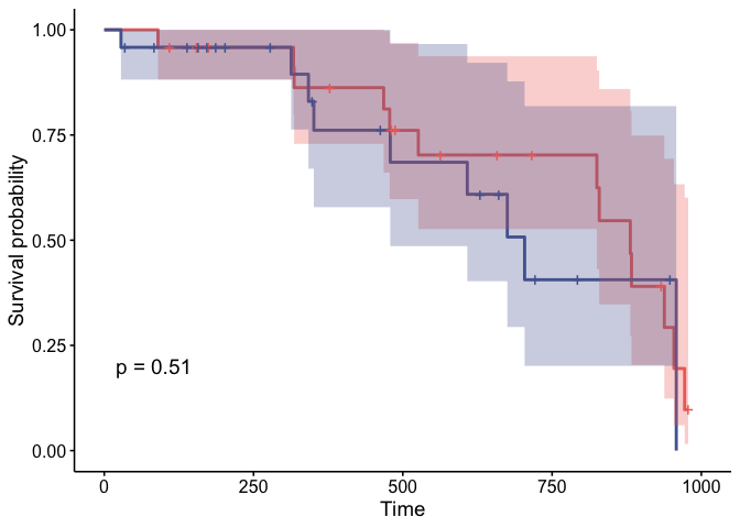

Cluster samples

We may want to cluster our data (e.g., using k-means sample-wise). cluster_elements takes as arguments a tibble, column names (as symbols; for sample, transcript and count) and returns a tibble with additional columns for the cluster annotation. At the moment only k-means clustering is supported, the plan is to introduce more clustering methods.

k-means

TidyTranscriptomics

counts_SE.norm.cluster = counts_SE.norm.MDS %>%
  cluster_elements(method="kmeans", centers = 2, action="get" )

Standard procedure (comparative purpose)

count_m_log = log(count_m + 1)

k = kmeans(count_m_log, iter.max = 1000, ...)
cluster = k$cluster

cluster$cell_type = tibble_counts[
    match(tibble_counts$sample, rownames(cluster)),
    c("Cell.type", "Dim1", "Dim2")
]

We can add cluster annotation to the MDS dimension reduced data set and plot.

 counts_SE.norm.cluster %>%
    ggplot(aes(x=`Dim1`, y=`Dim2`, color=`cluster_kmeans`)) +
  geom_point() +
  my_theme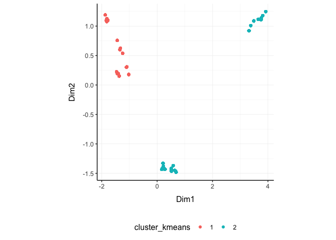

SNN

Matrix package (v1.3-3) causes an error with Seurat::FindNeighbors used in this method. We are trying to solve this issue. At the moment this option in unaviable.

TidyTranscriptomics

counts_SE.norm.SNN =
    counts_SE.norm.tSNE %>%
    cluster_elements(method = "SNN")

Standard procedure (comparative purpose)

library(Seurat)

snn = CreateSeuratObject(count_m)
snn = ScaleData(
    snn, display.progress = TRUE,
    num.cores=4, do.par = TRUE
)
snn = FindVariableFeatures(snn, selection.method = "vst")
snn = FindVariableFeatures(snn, selection.method = "vst")
snn = RunPCA(snn, npcs = 30)
snn = FindNeighbors(snn)
snn = FindClusters(snn, method = "igraph", ...)
snn = snn[["seurat_clusters"]]

snn$cell_type = tibble_counts[
    match(tibble_counts$sample, rownames(snn)),
    c("Cell.type", "Dim1", "Dim2")
]

counts_SE.norm.SNN %>%
    pivot_sample() %>%
    select(contains("tSNE"), everything()) 

counts_SE.norm.SNN %>%
    pivot_sample() %>%
    gather(source, Call, c("cluster_SNN", "Call")) %>%
    distinct() %>%
    ggplot(aes(x = `tSNE1`, y = `tSNE2`, color=Call)) + geom_point() + facet_grid(~source) + my_theme


# Do differential transcription between clusters
counts_SE.norm.SNN %>%
    mutate(factor_of_interest = `cluster_SNN` == 3) %>%
    test_differential_abundance(
    ~ factor_of_interest,
    action="get"
   )

Drop redundant transcripts

We may want to remove redundant elements from the original data set (e.g., samples or transcripts), for example if we want to define cell-type specific signatures with low sample redundancy. remove_redundancy takes as arguments a tibble, column names (as symbols; for sample, transcript and count) and returns a tibble with redundant elements removed (e.g., samples). Two redundancy estimation approaches are supported:

• removal of highly correlated clusters of elements (keeping a representative) with method=“correlation”
• removal of most proximal element pairs in a reduced dimensional space.

Approach 1

TidyTranscriptomics

counts_SE.norm.non_redundant =
    counts_SE.norm.MDS %>%
  remove_redundancy(    method = "correlation" )

## 
## The downloaded binary packages are in
##  /var/folders/zn/m_qvr9zd7tq0wdtsbq255f8xypj_zg/T//RtmpIi5KN6/downloaded_packages

Standard procedure (comparative purpose)

library(widyr)

.data.correlated =
    pairwise_cor(
        counts,
        sample,
        transcript,
        rc,
        sort = TRUE,
        diag = FALSE,
        upper = FALSE
    ) %>%
    filter(correlation > correlation_threshold) %>%
    distinct(item1) %>%
    rename(!!.element := item1)

# Return non redudant data frame
counts %>% anti_join(.data.correlated) %>%
    spread(sample, rc, - transcript) %>%
    left_join(annotation)

We can visualise how the reduced redundancy with the reduced dimentions look like

counts_SE.norm.non_redundant %>%
    pivot_sample() %>%
    ggplot(aes(x=`Dim1`, y=`Dim2`, color=`Cell.type`)) +
  geom_point() +
  my_theme

Approach 2

counts_SE.norm.non_redundant =
    counts_SE.norm.MDS %>%
  remove_redundancy(
    method = "reduced_dimensions",
    Dim_a_column = `Dim1`,
    Dim_b_column = `Dim2`
  )

We can visualise MDS reduced dimensions of the samples with the closest pair removed.

counts_SE.norm.non_redundant %>%
    pivot_sample() %>%
    ggplot(aes(x=`Dim1`, y=`Dim2`, color=`Cell.type`)) +
  geom_point() +
  my_theme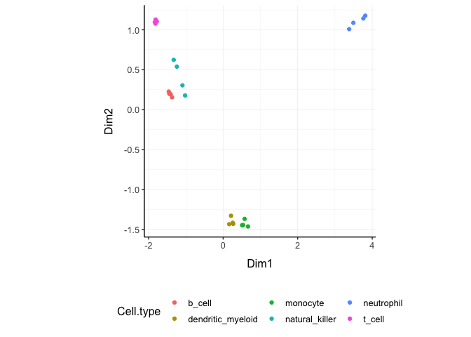

Other useful wrappers

The above wrapper streamline the most common processing of bulk RNA sequencing data. Other useful wrappers are listed above.

From BAM/SAM to tibble of gene counts

We can calculate gene counts (using FeatureCounts; Liao Y et al., 10.1093/nar/gkz114) from a list of BAM/SAM files and format them into a tidy structure (similar to counts).

counts = tidybulk_SAM_BAM(
    file_names,
    genome = "hg38",
    isPairedEnd = TRUE,
    requireBothEndsMapped = TRUE,
    checkFragLength = FALSE,
    useMetaFeatures = TRUE
)

From ensembl IDs to gene symbol IDs

We can add gene symbols from ensembl identifiers. This is useful since different resources use ensembl IDs while others use gene symbol IDs. This currently works for human and mouse.

counts_ensembl %>% ensembl_to_symbol(ens)

## # A tibble: 119 × 8
##    ens             iso   `read count` sample     cases…¹ cases…² trans…³ ref_g…⁴
##    <chr>           <chr>        <dbl> <chr>      <chr>   <chr>   <chr>   <chr>  
##  1 ENSG00000000003 13             144 TARGET-20… Acute … Primar… TSPAN6  hg38   
##  2 ENSG00000000003 13              72 TARGET-20… Acute … Primar… TSPAN6  hg38   
##  3 ENSG00000000003 13               0 TARGET-20… Acute … Primar… TSPAN6  hg38   
##  4 ENSG00000000003 13            1099 TARGET-20… Acute … Primar… TSPAN6  hg38   
##  5 ENSG00000000003 13              11 TARGET-20… Acute … Primar… TSPAN6  hg38   
##  6 ENSG00000000003 13               2 TARGET-20… Acute … Primar… TSPAN6  hg38   
##  7 ENSG00000000003 13               3 TARGET-20… Acute … Primar… TSPAN6  hg38   
##  8 ENSG00000000003 13            2678 TARGET-20… Acute … Primar… TSPAN6  hg38   
##  9 ENSG00000000003 13             751 TARGET-20… Acute … Primar… TSPAN6  hg38   
## 10 ENSG00000000003 13               1 TARGET-20… Acute … Primar… TSPAN6  hg38   
## # … with 109 more rows, and abbreviated variable names
## #   ¹​cases_0_project_disease_type, ²​cases_0_samples_0_sample_type, ³​transcript,
## #   ⁴​ref_genome
## # ℹ Use `print(n = ...)` to see more rows

From gene symbol to gene description (gene name in full)

We can add gene full name (and in future description) from symbol identifiers. This currently works for human and mouse.

counts_SE %>% 
    describe_transcript() %>% 
    select(feature, description, everything())

## # A SummarizedExperiment-tibble abstraction: 408,624 × 48
## # [90mFeatures=8513 | Samples=48 | Assays=count[0m
##    feature  sample     count Cell.…¹ time  condi…² batch facto…³ descr…⁴ gene_…⁵
##    <chr>    <chr>      <dbl> <fct>   <fct> <lgl>   <fct> <lgl>   <chr>   <chr>  
##  1 A1BG     SRR1740034   153 b_cell  0 d   TRUE    0     TRUE    alpha-… A1BG   
##  2 A1BG-AS1 SRR1740034    83 b_cell  0 d   TRUE    0     TRUE    A1BG a… A1BG-A…
##  3 AAAS     SRR1740034   868 b_cell  0 d   TRUE    0     TRUE    aladin… AAAS   
##  4 AACS     SRR1740034   222 b_cell  0 d   TRUE    0     TRUE    acetoa… AACS   
##  5 AAGAB    SRR1740034   590 b_cell  0 d   TRUE    0     TRUE    alpha … AAGAB  
##  6 AAMDC    SRR1740034    48 b_cell  0 d   TRUE    0     TRUE    adipog… AAMDC  
##  7 AAMP     SRR1740034  1257 b_cell  0 d   TRUE    0     TRUE    angio … AAMP   
##  8 AANAT    SRR1740034   284 b_cell  0 d   TRUE    0     TRUE    aralky… AANAT  
##  9 AAR2     SRR1740034   379 b_cell  0 d   TRUE    0     TRUE    AAR2 s… AAR2   
## 10 AARS2    SRR1740034   685 b_cell  0 d   TRUE    0     TRUE    alanyl… AARS2  
## # … with 40 more rows, and abbreviated variable names ¹​Cell.type, ²​condition,
## #   ³​factor_of_interest, ⁴​description, ⁵​gene_name
## # ℹ Use `print(n = ...)` to see more rows