10X Single cell sequencing data analysis - Chinese
Yue You
Luyi Tian
Source:vignettes/sc_analysis.Rmd
sc_analysis.RmdDescription
In this workshop (presented in Mandarin), you will learn how to analyse single-cell RNA-sequencing count data produced by the Chromium 10x platform using R/Bioconductor. This will include reading the data into R, pre-processing data, normalization, feature selection, dimensionality reduction and downstream analysis, such as clustering and cell type annotation.
Expectation: You will learn how to generate common plots for analysis and visualisation of single cell gene expfression data, such as diagnostic plots to assess the data quality as well as dimensionality reduction techniques such as principal components analysis and t-distributed stochastic neighbourhood embedding (t-SNE). The material we will be covering on single-cell RNA-sequencing analysis is a subset of the work of Amerzquita et al. (2020) Nature Methods,17:137–145 available at https://osca.bioconductor.org.
Pre-requisites: The course is aimed at PhD students, Master’s students, and third & fourth year undergraduate students. Some basic R knowledge is assumed - this is not an introduction to R course. If you are not familiar with the R statistical programming language it is compulsory that you work through an introductory R course before you attend this workshop.
Participation
After the lecture, participants are expected to follow along the hands-on session. we highly recommend participants bringing your own laptop.
数据准备
读取10xPBMC4k数据。
#--- loading ---#
unzip(system.file("extdata", "pbmc4k.zip", package = "zhejiang2020"),exdir = ".")

library(DropletUtils)
## Loading required package: SingleCellExperiment## Loading required package: SummarizedExperiment## Loading required package: MatrixGenerics## Loading required package: matrixStats##
## Attaching package: 'MatrixGenerics'## The following objects are masked from 'package:matrixStats':
##
## colAlls, colAnyNAs, colAnys, colAvgsPerRowSet, colCollapse,
## colCounts, colCummaxs, colCummins, colCumprods, colCumsums,
## colDiffs, colIQRDiffs, colIQRs, colLogSumExps, colMadDiffs,
## colMads, colMaxs, colMeans2, colMedians, colMins, colOrderStats,
## colProds, colQuantiles, colRanges, colRanks, colSdDiffs, colSds,
## colSums2, colTabulates, colVarDiffs, colVars, colWeightedMads,
## colWeightedMeans, colWeightedMedians, colWeightedSds,
## colWeightedVars, rowAlls, rowAnyNAs, rowAnys, rowAvgsPerColSet,
## rowCollapse, rowCounts, rowCummaxs, rowCummins, rowCumprods,
## rowCumsums, rowDiffs, rowIQRDiffs, rowIQRs, rowLogSumExps,
## rowMadDiffs, rowMads, rowMaxs, rowMeans2, rowMedians, rowMins,
## rowOrderStats, rowProds, rowQuantiles, rowRanges, rowRanks,
## rowSdDiffs, rowSds, rowSums2, rowTabulates, rowVarDiffs, rowVars,
## rowWeightedMads, rowWeightedMeans, rowWeightedMedians,
## rowWeightedSds, rowWeightedVars## Loading required package: GenomicRanges## Loading required package: stats4## Loading required package: BiocGenerics## Loading required package: parallel##
## Attaching package: 'BiocGenerics'## The following objects are masked from 'package:parallel':
##
## clusterApply, clusterApplyLB, clusterCall, clusterEvalQ,
## clusterExport, clusterMap, parApply, parCapply, parLapply,
## parLapplyLB, parRapply, parSapply, parSapplyLB## The following objects are masked from 'package:stats':
##
## IQR, mad, sd, var, xtabs## The following objects are masked from 'package:base':
##
## anyDuplicated, append, as.data.frame, basename, cbind, colnames,
## dirname, do.call, duplicated, eval, evalq, Filter, Find, get, grep,
## grepl, intersect, is.unsorted, lapply, Map, mapply, match, mget,
## order, paste, pmax, pmax.int, pmin, pmin.int, Position, rank,
## rbind, Reduce, rownames, sapply, setdiff, sort, table, tapply,
## union, unique, unsplit, which.max, which.min## Loading required package: S4Vectors##
## Attaching package: 'S4Vectors'## The following object is masked from 'package:base':
##
## expand.grid## Loading required package: IRanges## Loading required package: GenomeInfoDb## Loading required package: Biobase## Welcome to Bioconductor
##
## Vignettes contain introductory material; view with
## 'browseVignettes()'. To cite Bioconductor, see
## 'citation("Biobase")', and for packages 'citation("pkgname")'.##
## Attaching package: 'Biobase'## The following object is masked from 'package:MatrixGenerics':
##
## rowMedians## The following objects are masked from 'package:matrixStats':
##
## anyMissing, rowMedians
fname <- "pbmc4k"
sce.pbmc <- read10xCounts(fname, col.names=TRUE)
质量控制。
由于10x 技术会使得外部RNA,也就是不包含微滴的里的细胞被同时测序。在分析之前,我们需要确保得到的barcode数据都相对应活细胞。 这里,我们使用emptyDrops来筛选“真”细胞。
#--- cell-detection ---#
set.seed(100)
e.out <- emptyDrops(counts(sce.pbmc))
sce.pbmc <- sce.pbmc[,which(e.out$FDR <= 0.001)]
对于得到的基因,根据gene ID 进行基因注释,得到基因名,并且知道其所在染色体(用于之后的细胞质量控制)。
## Loading required package: ggplot2
rownames(sce.pbmc) <- uniquifyFeatureNames(
    rowData(sce.pbmc)$ID, rowData(sce.pbmc)$Symbol)

library(EnsDb.Hsapiens.v86)
## Loading required package: ensembldb## Loading required package: GenomicFeatures## Loading required package: AnnotationDbi## Loading required package: AnnotationFilter##
## Attaching package: 'ensembldb'## The following object is masked from 'package:stats':
##
## filter
location <- mapIds(EnsDb.Hsapiens.v86, keys=rowData(sce.pbmc)$ID,
    column="SEQNAME", keytype="GENEID")
## Warning: Unable to map 144 of 33694 requested IDs.
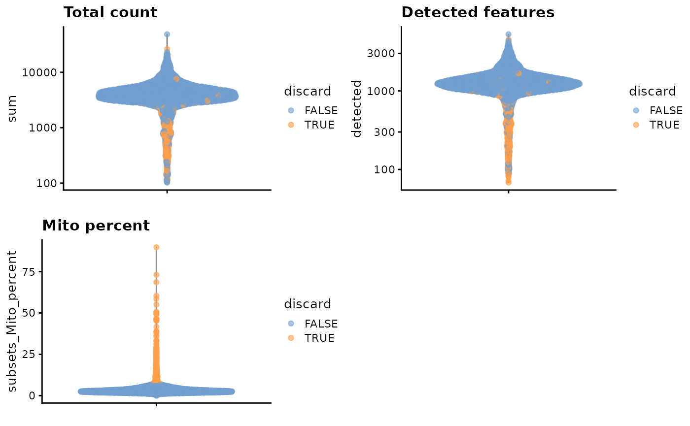
unfiltered <- sce.pbmc这里,我们认为线粒体基因表达量高的barcode对应细胞质mRNA已经流出的破损细胞。并用这个指标来进行筛查过滤。
#--- quality-control ---#
stats <- perCellQCMetrics(sce.pbmc, subsets=list(Mito=which(location=="MT")))
high.mito <- isOutlier(stats$subsets_Mito_percent, type="higher")
sce.pbmc <- sce.pbmc[,!high.mito]
summary(high.mito)## Mode FALSE TRUE
## logical 3985 315
colData(unfiltered) <- cbind(colData(unfiltered), stats)
unfiltered$discard <- high.mito

gridExtra::grid.arrange(
    plotColData(unfiltered, y="sum", colour_by="discard") +
        scale_y_log10() + ggtitle("Total count"),
    plotColData(unfiltered, y="detected", colour_by="discard") +
        scale_y_log10() + ggtitle("Detected features"),
    plotColData(unfiltered, y="subsets_Mito_percent",
        colour_by="discard") + ggtitle("Mito percent"),
    ncol=2
)
plotColData(unfiltered, x="sum", y="subsets_Mito_percent",
    colour_by="discard") + scale_x_log10()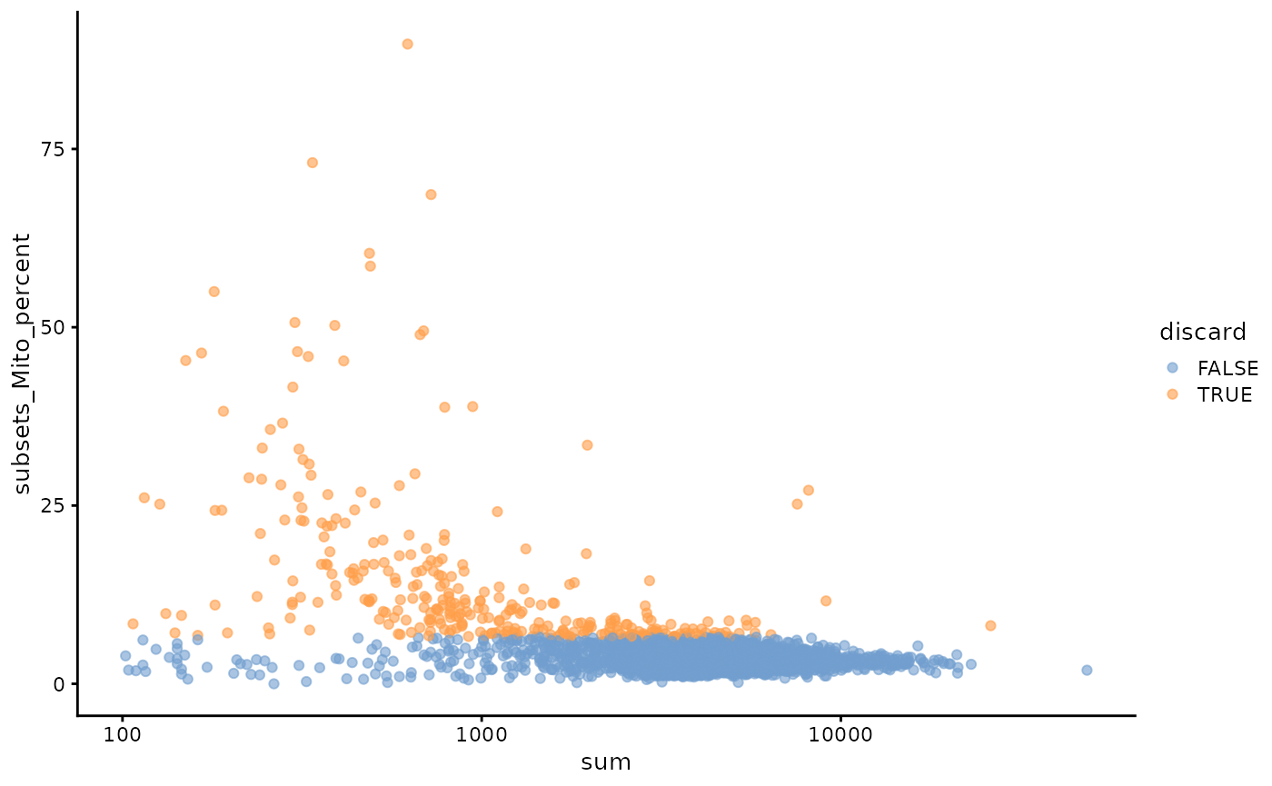
数据标准化
由于在mRNA分子的捕获,逆转录,测序过程中存在一定的技术误差,相同细胞的计数深度可能不相同。我们需要在进行细胞之间的比对之前,先尽可能的排除采样效应。进行数据标准化,使得细胞之间存在可比性。这里我们使用scran(Lun et al,2016a),一种允许更多细胞异质性的方法。
#--- normalization ---#
library(scran)
set.seed(1000)
clusters <- quickCluster(sce.pbmc)
sce.pbmc <- computeSumFactors(sce.pbmc, cluster=clusters)
sce.pbmc <- logNormCounts(sce.pbmc)
summary(sizeFactors(sce.pbmc))## Min. 1st Qu. Median Mean 3rd Qu. Max.
## 0.00749 0.71207 0.87490 1.00000 1.09900 12.25412特征选择
为了减轻下游分析工具的计算负担,减少数据中的噪声,我们需要先进行特征选择。
#--- variance-modelling ---#
set.seed(1001)
dec.pbmc <- modelGeneVarByPoisson(sce.pbmc)
top.pbmc <- getTopHVGs(dec.pbmc, prop=0.1)
plot(dec.pbmc$mean, dec.pbmc$total, pch=16, cex=0.5,
    xlab="Mean of log-expression", ylab="Variance of log-expression")
curfit <- metadata(dec.pbmc)
curve(curfit$trend(x), col='dodgerblue', add=TRUE, lwd=2)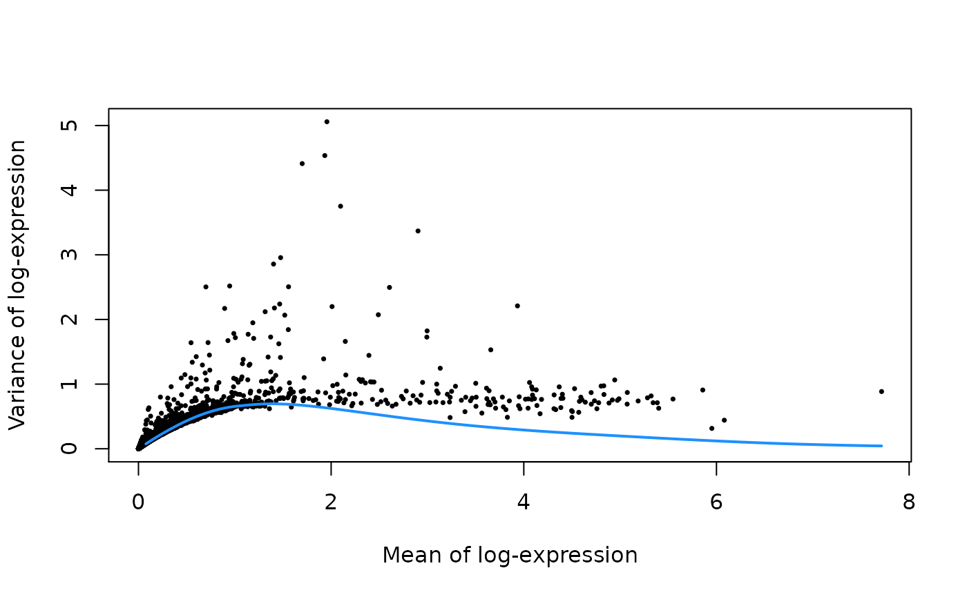
特征选择后,单细胞表达矩阵的维数可以通过专门的降维算法进一步降低。使得数据可以直观可视化,并且将数据简化为基本组成部分。
#--- dimensionality-reduction ---#
set.seed(10000)
sce.pbmc <- denoisePCA(sce.pbmc, subset.row=top.pbmc, technical=dec.pbmc)

set.seed(100000)
sce.pbmc <- runTSNE(sce.pbmc, dimred="PCA")

set.seed(1000000)
sce.pbmc <- runUMAP(sce.pbmc, dimred="PCA")
ncol(reducedDim(sce.pbmc, "PCA"))## [1] 9聚类分析
使用louvain算法进行聚类
louvain算法是一个基于图的聚类算法,我们首先构建Shared Nearest Neighbor(SNN)图,输入为使用主成分分析(PCA)降维后得到的矩阵。 在得到SNN图g之后,我们使用它作为louvain算法的输入。
g <- buildSNNGraph(sce.pbmc, k=10, use.dimred = 'PCA')
clust <- igraph::cluster_louvain(g)$membership

sce.pbmc$cluster <- factor(clust)
table(clust)
## clust
## 1 2 3 4 5 6 7 8 9 10 11 12 13 14
## 353 152 376 857 48 46 68 661 287 53 541 198 219 126使用tSNE对聚类进行可视化。
plotTSNE(sce.pbmc, colour_by="cluster",text_by="cluster")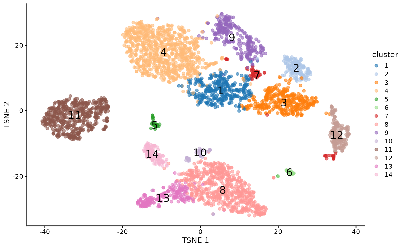
使用UMAP对聚类进行可视化。
plotUMAP(sce.pbmc, colour_by="cluster",text_by="cluster")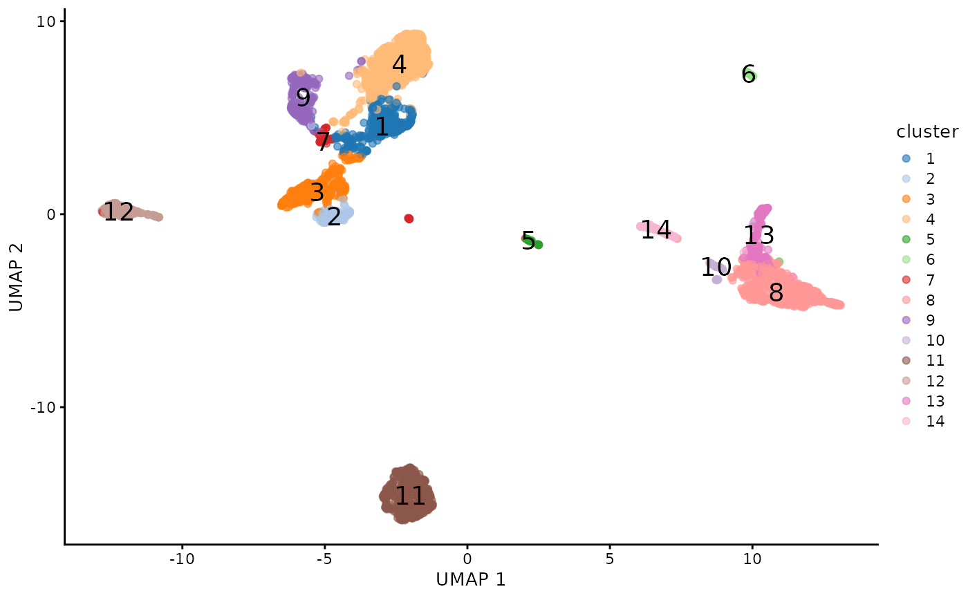
寻找聚类特异表达基因
在获得了聚类之后,我们想要知道每个聚类都哪些高表达的基因,这些基因往往是能区分不同细胞类型的marker gene,也可以帮助我们了解不同聚类的生物学功能。
library(RColorBrewer)这里,我们通过比对某一cluster和其他所有cluster的表达来找到marker gene, 并且只挑选显示上调基因。
markers.pbmc <- findMarkers(sce.pbmc, sce.pbmc$cluster,
    pval.type="all", direction="up")
markers.pbmc[[1]][order(markers.pbmc[[1]]$FDR),]## DataFrame with 33694 rows and 16 columns
## p.value FDR summary.logFC logFC.2 logFC.3
## <numeric> <numeric> <numeric> <numeric> <numeric>
## LTB 4.74177e-07 0.0159769 0.364873 1.727152 2.003863
## TRADD 3.34176e-05 0.5629862 0.246261 0.246261 0.358697
## TNFAIP3 3.64851e-04 1.0000000 0.294551 0.586788 0.324352
## RP11-138A9.1 5.51754e-04 1.0000000 0.235830 0.265198 0.204199
## CD69 9.05928e-04 1.0000000 0.220119 0.889346 0.220119
## ... ... ... ... ... ...
## RP11-1143G9.4 1 1 -2.88441 0.0632559 0.04136662
## CD79B 1 1 -2.65518 -0.0319757 0.04062722
## CST3 1 1 -3.38955 0.1132112 -0.00139546
## TYROBP 1 1 -3.77926 -0.2135870 -0.12432406
## CD79A 1 1 -2.88958 0.0547465 0.02026294
## logFC.4 logFC.5 logFC.6 logFC.7 logFC.8
## <numeric> <numeric> <numeric> <numeric> <numeric>
## LTB 0.709584 2.236589 3.179486 1.384048 3.011681
## TRADD 0.455837 0.399715 0.625041 0.340638 0.494083
## TNFAIP3 0.386801 0.634728 0.640136 0.539046 0.355789
## RP11-138A9.1 0.297797 0.338809 0.459562 0.235830 0.436762
## CD69 0.182859 1.453419 1.796272 0.809607 1.625559
## ... ... ... ... ... ...
## RP11-1143G9.4 0.02079562 -0.0410564 -0.0987084 -0.0922961 -2.8844113
## CD79B 0.03988754 -0.0332708 0.0275658 -0.2155062 0.0970271
## CST3 -0.00267045 -2.1438978 -1.5534313 -0.1021948 -3.3895523
## TYROBP -0.04510738 -1.6678515 -0.4775968 0.0929494 -3.7792602
## CD79A -0.02744100 -0.1171942 0.0907275 -0.0144729 0.0329842
## logFC.9 logFC.10 logFC.11 logFC.12 logFC.13 logFC.14
## <numeric> <numeric> <numeric> <numeric> <numeric> <numeric>
## LTB 0.364873 1.564212 0.345040 2.919553 2.640417 2.967425
## TRADD 0.219922 0.466701 0.454696 0.485817 0.455422 0.358617
## TNFAIP3 0.573474 0.294551 0.641317 0.537594 0.548100 0.548964
## RP11-138A9.1 0.261783 0.382809 0.292954 0.393811 0.414021 0.436237
## CD69 1.210379 1.001879 0.441418 0.696360 1.577163 1.468100
## ... ... ... ... ... ... ...
## RP11-1143G9.4 0.0667527 -2.190784 0.0273067 0.0288028 -1.07943585 -1.7809210
## CD79B -0.0434586 -0.464497 -2.6551786 -0.0206008 -0.27267278 -0.0135700
## CST3 -0.0285401 -2.688015 0.0152875 0.1102020 -3.64978261 -4.3511281
## TYROBP -0.0414366 -3.077268 -0.0436713 -2.3635000 -3.65373554 -2.3592519
## CD79A 0.0118844 -0.347398 -2.8895764 0.0677690 -0.00864517 -0.0389843查看marker gene。
# NOTE: this is not efficient for large iteration.
marker_genes = c()

for (i in 1:length(markers.pbmc)){
  tmp = markers.pbmc[[i]][order(markers.pbmc[[i]]$FDR),]
  marker_genes = c(marker_genes, rownames(tmp)[1:5])
}

marker_genes = unique(marker_genes)
marker_genes
## [1] "LTB" "TRADD" "TNFAIP3" "RP11-138A9.1" "CD69"
## [6] "RORA" "KLRG1" "SESN1" "TRGC1" "LINC00987"
## [11] "DUSP2" "CD8A" "KLRC2" "CRTAM" "GADD45B"
## [16] "CCR7" "RPS13" "RPL35A" "RPL34" "RPL21"
## [21] "ITM2C" "LILRA4" "IRF7" "JCHAIN" "MZB1"
## [26] "PF4" "SDPR" "TMSB4X" "NRGN" "TAGLN2"
## [31] "TAP1" "DUSP4" "CTLA4" "FOXP3" "PTTG1"
## [36] "S100A6" "LYZ" "CSTA" "FCN1" "S100A9"
## [41] "GIMAP7" "MALAT1" "RPLP1" "GIMAP1" "GCC2"
## [46] "MBNL1" "NDUFB11" "NUFIP2" "ALPK1" "ZSWIM8"
## [51] "CD79A" "HLA-DOB" "VPREB3" "CD72" "CD79B"
## [56] "KLRF1" "PRF1" "SPON2" "FGFBP2" "GNLY"
## [61] "LST1" "IFITM3" "AIF1" "MS4A7" "SERPINA1"
## [66] "HLA-DRB1" "HLA-DQA1" "HLA-DPB1" "HLA-DRA" "HLA-DPA1"查看特定基因在不同cluster的表达量。
plotExpression(sce.pbmc, x="cluster",features="MS4A1")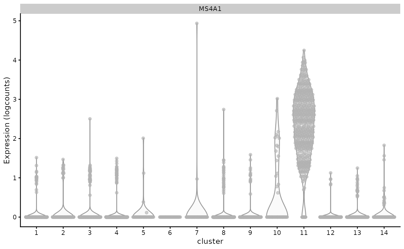
plotExpression(sce.pbmc, x="cluster",features="GZMK")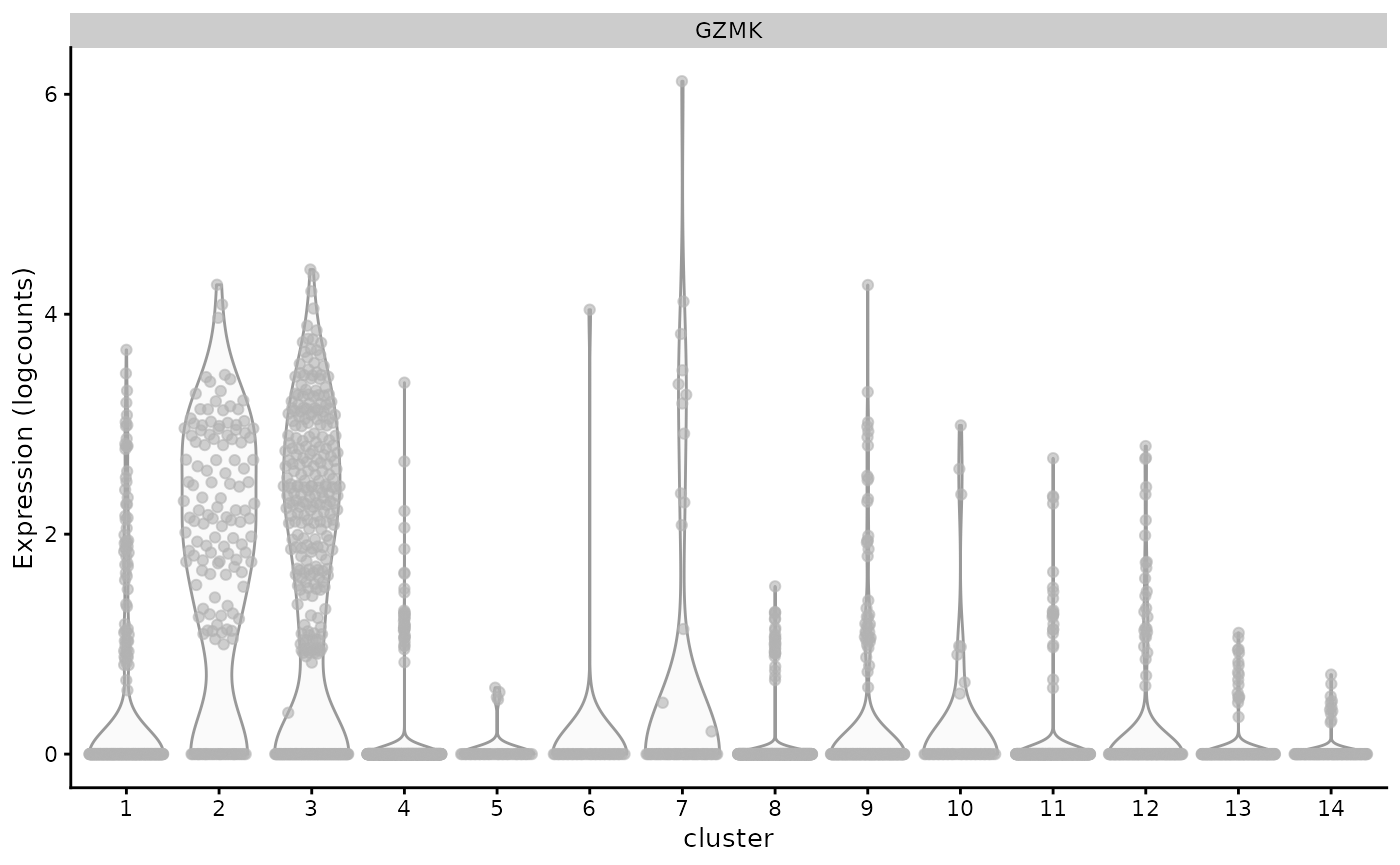
使用热图对marker gene进行可视化。
getPalette = colorRampPalette(brewer.pal(9, "Set1"))
anno_df = as.data.frame(colData(sce.pbmc))
anno_df = anno_df[,"cluster", drop=FALSE]


col_cluster = getPalette(nlevels(anno_df$cluster))

names(col_cluster) =  levels(anno_df$cluster)

annotation_colors = list(cluster=col_cluster)

tmp_expr = logcounts(sce.pbmc)[marker_genes,]
tmp_expr = t(scale(t(tmp_expr)))
tmp_expr[tmp_expr<(-2.5)]=-2.5
tmp_expr[tmp_expr>2.5]=2.5
colnames(tmp_expr) = colnames(sce.pbmc)

pheatmap::pheatmap(tmp_expr[,order(sce.pbmc$cluster)],
         cluster_cols = FALSE,
         cluster_rows = FALSE,
         annotation_col = anno_df,
         annotation_colors=annotation_colors,
         show_colnames = FALSE,
         fontsize_row=6)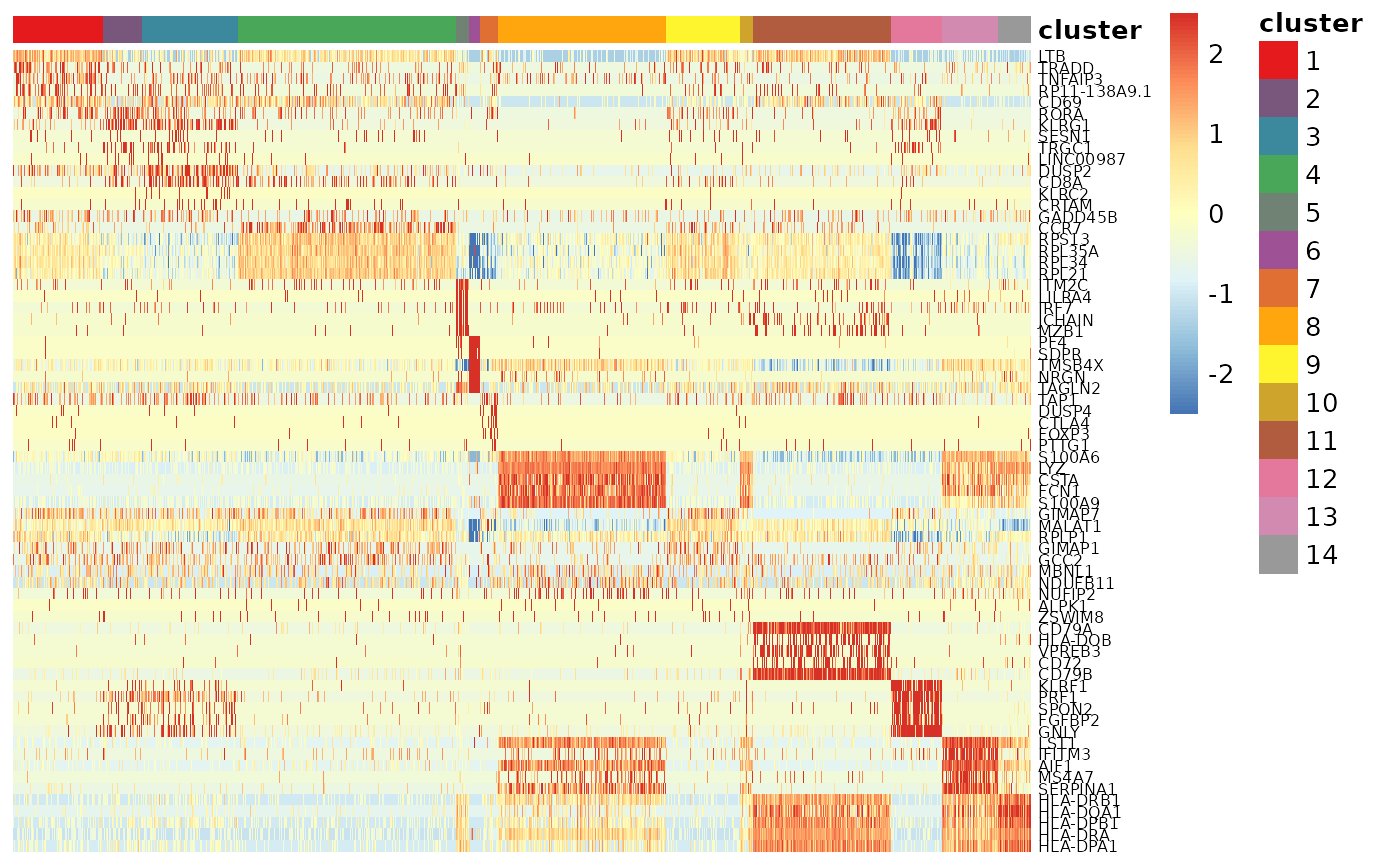
使用singleR进行细胞类型注释
我们选择 BlueprintEncodeData() 来作为参考数据。(Martens and Stunnenberg 2013; The ENCODE Project Consortium 2012)
ref <- BlueprintEncodeData()## Warning: 'BlueprintEncodeData' is deprecated.
## Use 'celldex::BlueprintEncodeData' instead.
## See help("Deprecated")## using temporary cache /tmp/RtmpubWEJY/BiocFileCache## snapshotDate(): 2020-10-02## see ?celldex and browseVignettes('celldex') for documentation## downloading 1 resources## retrieving 1 resource## loading from cache## see ?celldex and browseVignettes('celldex') for documentation## downloading 1 resources## retrieving 1 resource## loading from cache##
## B-cells CD4+ T-cells CD8+ T-cells DC Eosinophils Erythrocytes
## 549 773 1274 1 1 5
## HSC Monocytes NK cells
## 14 1117 251
plotScoreHeatmap(pred)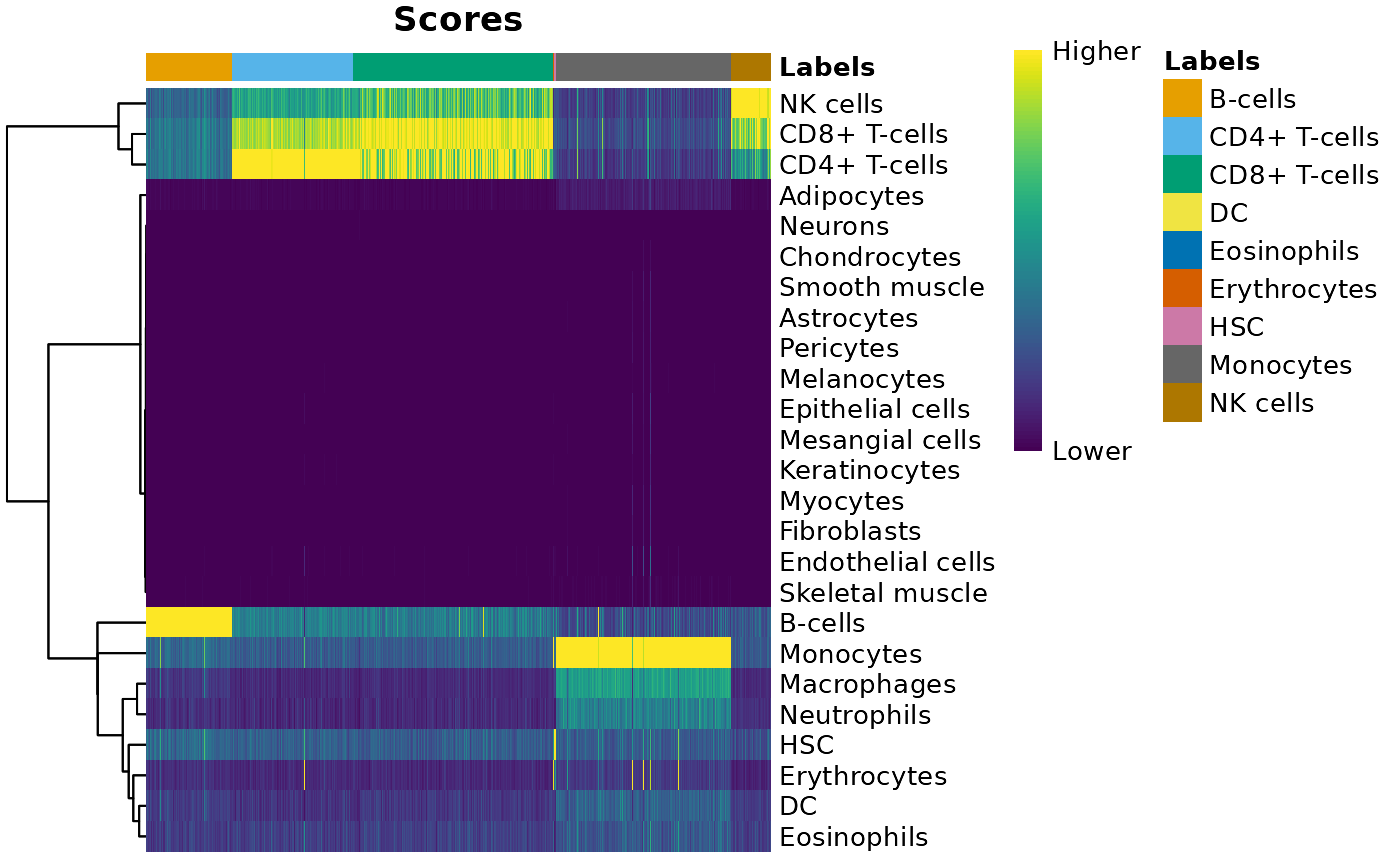
利用每个cluster和对每个细胞计算得到的可能细胞类型画heatmap。
tab <- table(Assigned=pred$pruned.labels, Cluster=sce.pbmc$cluster)

# Adding a pseudo-count of 10 to avoid strong color jumps with just 1 cell.
library(pheatmap)
pheatmap(log2(tab+10), color=colorRampPalette(c("white", "blue"))(101))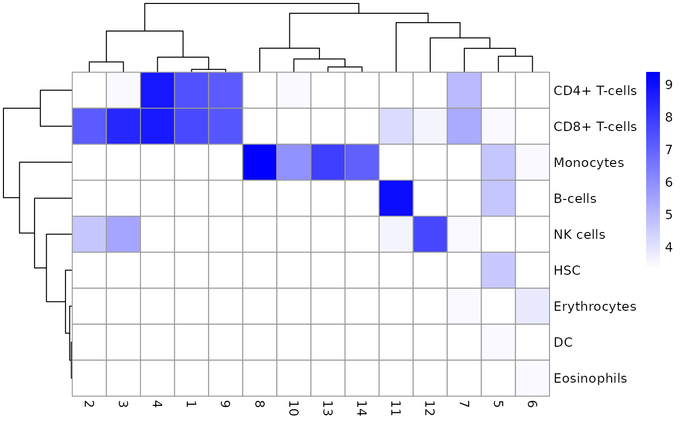
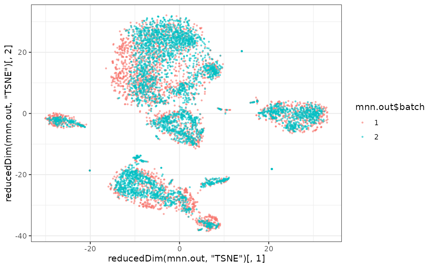
数据整合
这里我们使用MNN算法整合多个数据并消除批次效应(batch effects)
首先对两个PBMC单细胞数据集进行预处理
#--- loading ---#
library(TENxPBMCData)
## Loading required package: HDF5Array## Loading required package: DelayedArray## Loading required package: Matrix##
## Attaching package: 'Matrix'## The following object is masked from 'package:S4Vectors':
##
## expand##
## Attaching package: 'DelayedArray'## The following objects are masked from 'package:base':
##
## aperm, apply, rowsum## Loading required package: rhdf5
pbmc4k <- TENxPBMCData('pbmc4k')## snapshotDate(): 2020-10-02## see ?TENxPBMCData and browseVignettes('TENxPBMCData') for documentation## downloading 1 resources## retrieving 1 resource## loading from cache
#--- quality-control ---#
is.mito <- grep("MT", rowData(pbmc4k)$Symbol_TENx)

library(scater)
stats <- perCellQCMetrics(pbmc4k, subsets=list(Mito=is.mito))
high.mito <- isOutlier(stats$subsets_Mito_percent, type="higher")
pbmc4k <- pbmc4k[,!high.mito]

#--- normalization ---#
pbmc4k <- logNormCounts(pbmc4k)

#--- variance-modelling ---#
library(scran)
dec4k <- modelGeneVar(pbmc4k)
chosen.hvgs <- getTopHVGs(dec4k, prop=0.1)

#--- dimensionality-reduction ---#
set.seed(10000)
pbmc4k <- runPCA(pbmc4k, subset_row=chosen.hvgs, ncomponents=25,
    BSPARAM=BiocSingular::RandomParam())

set.seed(100000)
pbmc4k <- runTSNE(pbmc4k, dimred="PCA")

set.seed(1000000)
pbmc4k <- runUMAP(pbmc4k, dimred="PCA")

#--- clustering ---#
g <- buildSNNGraph(pbmc4k, k=10, use.dimred = 'PCA')
clust <- igraph::cluster_walktrap(g)$membership
pbmc4k$cluster <- factor(clust)
#--- loading ---#
library(TENxPBMCData)
pbmc3k <- TENxPBMCData('pbmc3k')
## snapshotDate(): 2020-10-02## see ?TENxPBMCData and browseVignettes('TENxPBMCData') for documentation## downloading 1 resources## retrieving 1 resource## loading from cache
#--- quality-control ---#
is.mito <- grep("MT", rowData(pbmc3k)$Symbol_TENx)

library(scater)
stats <- perCellQCMetrics(pbmc3k, subsets=list(Mito=is.mito))
high.mito <- isOutlier(stats$subsets_Mito_percent, type="higher")
pbmc3k <- pbmc3k[,!high.mito]

#--- normalization ---#
pbmc3k <- logNormCounts(pbmc3k)

#--- variance-modelling ---#
library(scran)
dec3k <- modelGeneVar(pbmc3k)
chosen.hvgs <- getTopHVGs(dec3k, prop=0.1)

#--- dimensionality-reduction ---#
set.seed(10000)
pbmc3k <- runPCA(pbmc3k, subset_row=chosen.hvgs, ncomponents=25,
    BSPARAM=BiocSingular::RandomParam())

set.seed(100000)
pbmc3k <- runTSNE(pbmc3k, dimred="PCA")

set.seed(1000000)
pbmc3k <- runUMAP(pbmc3k, dimred="PCA")

#--- clustering ---#
g <- buildSNNGraph(pbmc3k, k=10, use.dimred = 'PCA')
clust <- igraph::cluster_louvain(g)$membership
pbmc3k$cluster <- factor(clust)
由于两个数据集所表达的基因不尽相同,我们取两个数据集表达基因的交集并且过滤掉不同的基因,以保证两个数据集的每一行都是一样的基因。
## [1] 31232
# Subsetting the SingleCellExperiment object.
pbmc3k <- pbmc3k[universe,]
pbmc4k <- pbmc4k[universe,]

# Also subsetting the variance modelling results, for convenience.
dec3k <- dec3k[universe,]
dec4k <- dec4k[universe,]
combined.dec <- combineVar(dec3k, dec4k)
chosen.hvgs <- combined.dec$bio > 0
sum(chosen.hvgs)
## [1] 13431
library(batchelor)
rescaled <- multiBatchNorm(pbmc3k, pbmc4k)
pbmc3k <- rescaled[[1]]
pbmc4k <- rescaled[[2]]
# Synchronizing the metadata for cbind()ing.
rowData(pbmc3k) <- rowData(pbmc4k)
colData(pbmc3k) = colData(pbmc3k)[,colnames(colData(pbmc4k))]
pbmc3k$batch <- "3k"
pbmc4k$batch <- "4k"
uncorrected <- cbind(pbmc3k,pbmc4k)

# Using RandomParam() as it is more efficient for file-backed matrices.
library(scater)
uncorrected <- runPCA(uncorrected, subset_row=chosen.hvgs,
    BSPARAM=BiocSingular::RandomParam())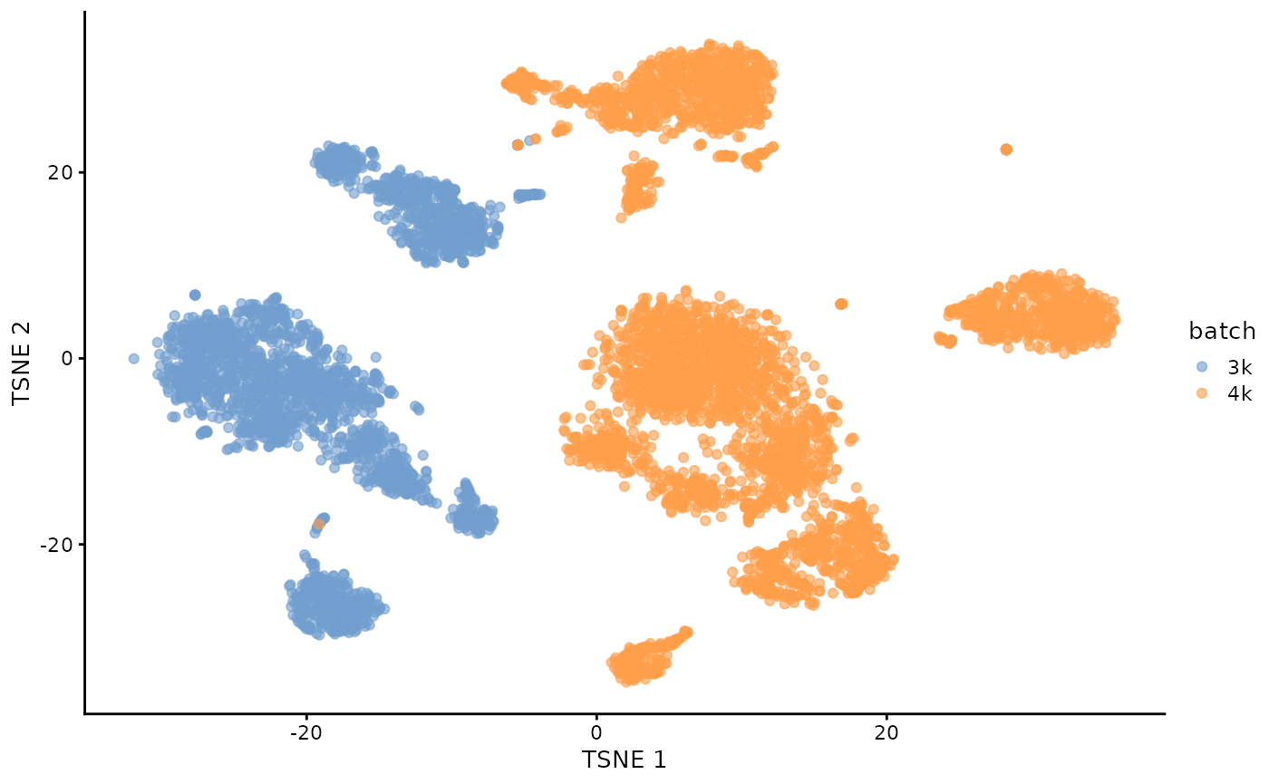
# Using randomized SVD here, as this is faster than
# irlba for file-backed matrices.
mnn.out <- fastMNN(pbmc3k, pbmc4k, d=50, k=20, subset.row=chosen.hvgs,
    BSPARAM=BiocSingular::RandomParam(deferred=TRUE))
mnn.out
## class: SingleCellExperiment
## dim: 13431 6791
## metadata(2): merge.info pca.info
## assays(1): reconstructed
## rownames(13431): ENSG00000239945 ENSG00000228463 ... ENSG00000198695
## ENSG00000198727
## rowData names(1): rotation
## colnames: NULL
## colData names(1): batch
## reducedDimNames(1): corrected
## altExpNames(0):
library(scater)
mnn.out <- runTSNE(mnn.out, dimred="corrected")

mnn.out$batch <- factor(mnn.out$batch)
plotTSNE(mnn.out, colour_by="batch")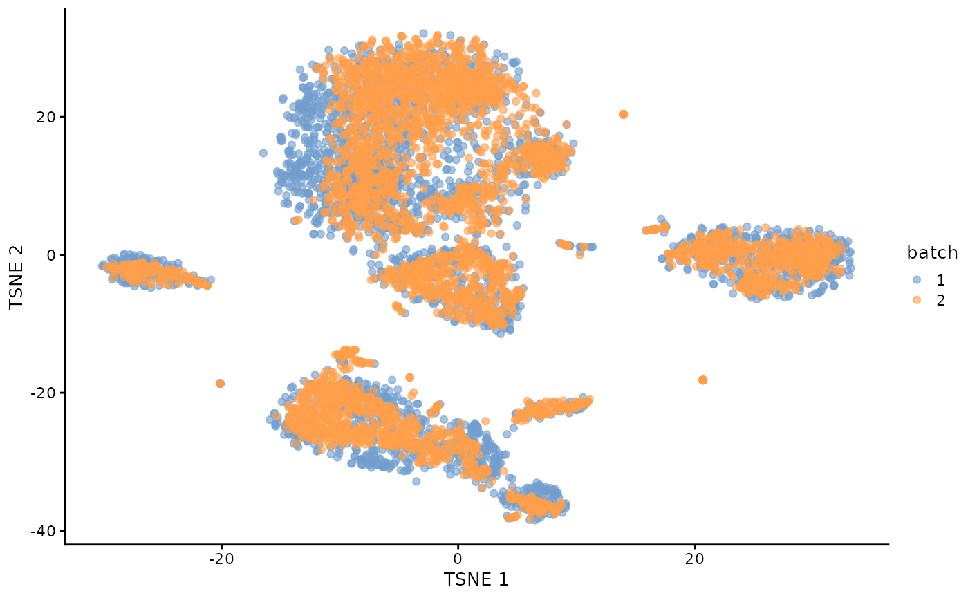
ggplot()+
  geom_point(alpha=0.5,size=0.5,aes(x=reducedDim(mnn.out,"TSNE")[,1],y=reducedDim(mnn.out,"TSNE")[,2],col=mnn.out$batch))+
  theme_bw()