Single-cell Tidy Transcriptomics - analysis of single-cell RNA sequencing data with R tidy principles
Stefano Mangiola
The Walter and Eliza Hall Institute of Medical Research, 1G Royal Parade, Parkville, VIC 3052, Melbourne, Australia; Department of Medical Biology, The University of Melbourne, Parkville, VIC 3010, Melbourne, AustraliaMaria Doyle
Peter MacCallum Cancer Centre, 305 Grattan Street, Parkville, Melbourne, Victoria, Australia11 November 2020
Source:vignettes/tidy_single_cell.Rmd
tidy_single_cell.Rmd![]()
Set-up
library(zhejiang2020)

# Bioconductor
library(scran)
library(scater)
library(EnsDb.Hsapiens.v86)

# tidyverse core packages
library(tibble)
library(dplyr)
library(tidyr)
library(readr)
library(magrittr)
library(ggplot2)
library(ggbeeswarm)

#library(tidyHeatmap)
library(SingleCellExperiment)
library(tidySingleCellExperiment)
Participation
After the lecture, participants are expected to follow along the hands-on session. we highly recommend participants bringing your own laptop.
R / Bioconductor packages used
The following R/Bioconductor packages will be explicitly used:
- tidySingleCellExperiment
- DropletUtils
- scran
- scater
- singleR
Data loading
We get the original SingleCellExperiment data used in the previous session.
zhejiang2020::single_cell_experiment## class: SingleCellExperiment
## dim: 33694 4290
## metadata(1): Samples
## assays(1): counts
## rownames(33694): ENSG00000243485 ENSG00000237613 ... ENSG00000277475
## ENSG00000268674
## rowData names(2): ID Symbol
## colnames(4290): AAACCTGAGAAGGCCT-1 AAACCTGAGACAGACC-1 ...
## TTTGTCAGTTAAGACA-1 TTTGTCATCCCAAGAT-1
## colData names(2): Sample Barcode
## reducedDimNames(0):
## altExpNames(0):We can get a tidy representation where cell-wise information is displayed. The dataframe is displayed as tibble abstraction, to indicate that appears and act as a tibble, but underlies a SingleCellExperiment.
counts =
  zhejiang2020::single_cell_experiment %>%
  tidy()

counts
## # A tibble abstraction: 4,290 x 3
## cell Sample Barcode
## <chr> <chr> <chr>
## 1 AAACCTGAGAAGGCCT-1 raw_gene_bc_matrices/GRCh38 AAACCTGAGAAGGCCT-1
## 2 AAACCTGAGACAGACC-1 raw_gene_bc_matrices/GRCh38 AAACCTGAGACAGACC-1
## 3 AAACCTGAGATAGTCA-1 raw_gene_bc_matrices/GRCh38 AAACCTGAGATAGTCA-1
## 4 AAACCTGAGGCATGGT-1 raw_gene_bc_matrices/GRCh38 AAACCTGAGGCATGGT-1
## 5 AAACCTGCAAGGTTCT-1 raw_gene_bc_matrices/GRCh38 AAACCTGCAAGGTTCT-1
## 6 AAACCTGCAGGATTGG-1 raw_gene_bc_matrices/GRCh38 AAACCTGCAGGATTGG-1
## 7 AAACCTGCAGGCGATA-1 raw_gene_bc_matrices/GRCh38 AAACCTGCAGGCGATA-1
## 8 AAACCTGCATGAAGTA-1 raw_gene_bc_matrices/GRCh38 AAACCTGCATGAAGTA-1
## 9 AAACCTGGTAAATGAC-1 raw_gene_bc_matrices/GRCh38 AAACCTGGTAAATGAC-1
## 10 AAACCTGGTACATCCA-1 raw_gene_bc_matrices/GRCh38 AAACCTGGTACATCCA-1
## # … with 4,280 more rowsIf we need, we can extract transcript information too. A regular tibble will be returned for independent visualisation and analyses.
counts %>%
  join_transcripts("ENSG00000228463")
## tidySingleCellExperiment says: A data frame is returned for independent data analysis.## # A tibble: 4,290 x 5
## cell transcript abundance_counts Sample Barcode
## <chr> <chr> <dbl> <chr> <chr>
## 1 AAACCTGAGAAG… ENSG00000228… 0 raw_gene_bc_matri… AAACCTGAGAAG…
## 2 AAACCTGAGACA… ENSG00000228… 0 raw_gene_bc_matri… AAACCTGAGACA…
## 3 AAACCTGAGATA… ENSG00000228… 0 raw_gene_bc_matri… AAACCTGAGATA…
## 4 AAACCTGAGGCA… ENSG00000228… 0 raw_gene_bc_matri… AAACCTGAGGCA…
## 5 AAACCTGCAAGG… ENSG00000228… 0 raw_gene_bc_matri… AAACCTGCAAGG…
## 6 AAACCTGCAGGA… ENSG00000228… 0 raw_gene_bc_matri… AAACCTGCAGGA…
## 7 AAACCTGCAGGC… ENSG00000228… 0 raw_gene_bc_matri… AAACCTGCAGGC…
## 8 AAACCTGCATGA… ENSG00000228… 0 raw_gene_bc_matri… AAACCTGCATGA…
## 9 AAACCTGGTAAA… ENSG00000228… 0 raw_gene_bc_matri… AAACCTGGTAAA…
## 10 AAACCTGGTACA… ENSG00000228… 0 raw_gene_bc_matri… AAACCTGGTACA…
## # … with 4,280 more rowsAs before, we add gene symbols to the data
#--- gene-annotation ---#
rownames(counts) <-
  uniquifyFeatureNames(
    rowData(counts)$ID,
    rowData(counts)$Symbol
  )
We check the mitochondrial expression for all cells
# Gene product location
location <- mapIds(
  EnsDb.Hsapiens.v86,
  keys=rowData(counts)$ID,
  column="SEQNAME",
  keytype="GENEID"
)
## Warning: Unable to map 144 of 33694 requested IDs.
#--- quality-control ---#
counts_annotated =
  counts %>%

  # Join mitochondrion statistics
  left_join(
    perCellQCMetrics(., subsets=list(Mito=which(location=="MT"))) %>%
    as_tibble(rownames="cell"),
    by="cell"
  ) %>%

  # Label cells
  mutate(high_mitochondrion = isOutlier(subsets_Mito_percent, type="higher"))
We can plot various statistics
counts_annotated %>%
  plotColData(
    y = "subsets_Mito_percent",
    colour_by = "high_mitochondrion"
  ) +
  ggtitle("Mito percent")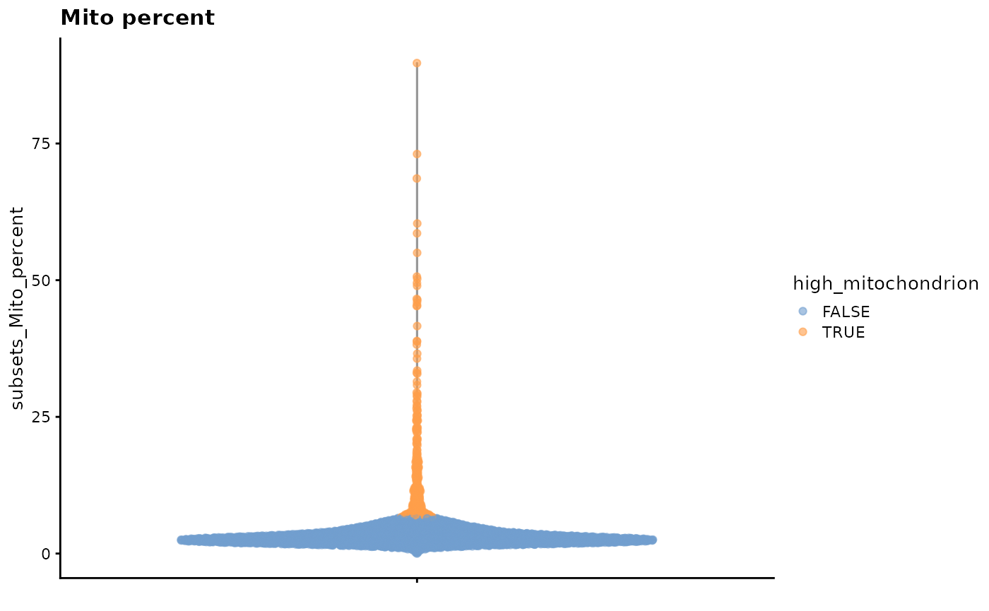
counts_annotated %>%
  ggplot(aes(x=1,y=subsets_Mito_percent,
             color = high_mitochondrion,
             alpha=high_mitochondrion,
             size= high_mitochondrion
            )) +
  ggbeeswarm::geom_quasirandom() +

  # Customisation
  scale_color_manual(values=c("black", "#e11f28")) +
  scale_size_discrete(range = c(0, 2))
## Warning: Using size for a discrete variable is not advised.## Warning: Using alpha for a discrete variable is not advised.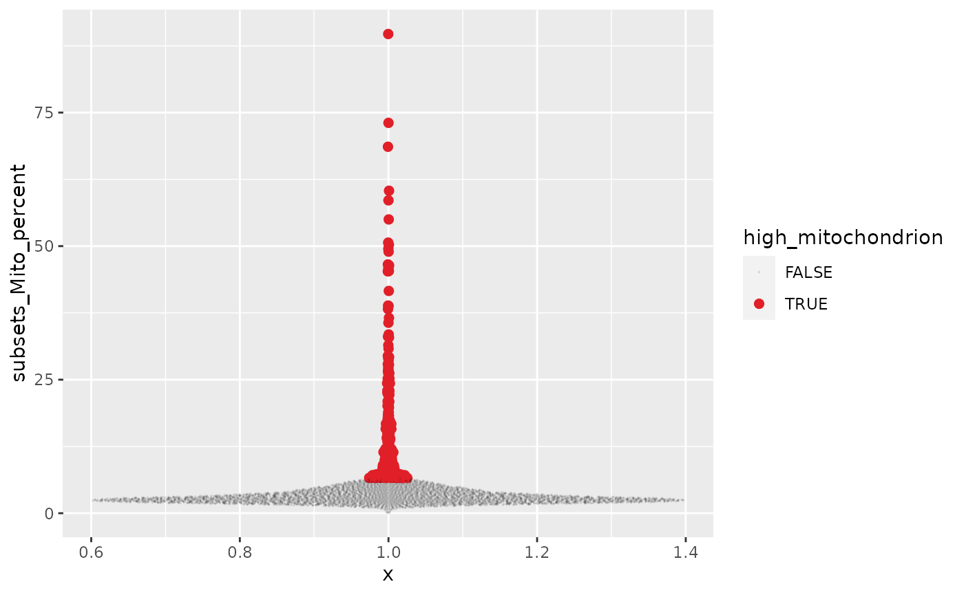
We can filter the the alive cells using dplyr function.
counts_filtered =
  counts_annotated %>%

  # Filter data
  filter(!high_mitochondrion)

counts_filtered
## # A tibble abstraction: 3,978 x 10
## cell Sample Barcode sum detected subsets_Mito_sum subsets_Mito_de…
## <chr> <chr> <chr> <dbl> <int> <dbl> <int>
## 1 AAAC… raw_g… AAACCT… 1738 748 111 11
## 2 AAAC… raw_g… AAACCT… 3240 1052 177 12
## 3 AAAC… raw_g… AAACCT… 2983 951 67 11
## 4 AAAC… raw_g… AAACCT… 4181 1248 93 10
## 5 AAAC… raw_g… AAACCT… 12147 2785 394 11
## 6 AAAC… raw_g… AAACCT… 8588 2278 385 11
## 7 AAAC… raw_g… AAACCT… 3158 1118 109 11
## 8 AAAC… raw_g… AAACCT… 5081 1437 90 10
## 9 AAAC… raw_g… AAACCT… 3562 970 66 11
## 10 AAAC… raw_g… AAACCT… 7157 1639 173 12
## # … with 3,968 more rows, and 3 more variables: subsets_Mito_percent <dbl>,
## # total <dbl>, high_mitochondrion <lgl>Scaling
As before, we can use standard Bioconductor utilities for calculating scaled log counts.
#--- normalization ---#
set.seed(1000)

# Calculate clusters
clusters <- quickCluster(counts_filtered)

# Add scaled counts
counts_scaled <-
  counts_filtered %>%
  computeSumFactors(cluster=clusters) %>%
  logNormCounts()

counts_scaled %>%
  join_transcripts("CD79B")
## tidySingleCellExperiment says: A data frame is returned for independent data analysis.## # A tibble: 3,978 x 14
## cell transcript abundance_counts abundance_logco… Sample Barcode sum
## <chr> <chr> <dbl> <dbl> <chr> <chr> <dbl>
## 1 AAAC… CD79B 0 0 raw_g… AAACCT… 1738
## 2 AAAC… CD79B 1 1.21 raw_g… AAACCT… 3240
## 3 AAAC… CD79B 0 0 raw_g… AAACCT… 2983
## 4 AAAC… CD79B 0 0 raw_g… AAACCT… 4181
## 5 AAAC… CD79B 0 0 raw_g… AAACCT… 12147
## 6 AAAC… CD79B 6 2.05 raw_g… AAACCT… 8588
## 7 AAAC… CD79B 4 2.75 raw_g… AAACCT… 3158
## 8 AAAC… CD79B 0 0 raw_g… AAACCT… 5081
## 9 AAAC… CD79B 0 0 raw_g… AAACCT… 3562
## 10 AAAC… CD79B 0 0 raw_g… AAACCT… 7157
## # … with 3,968 more rows, and 7 more variables: detected <int>,
## # subsets_Mito_sum <dbl>, subsets_Mito_detected <int>,
## # subsets_Mito_percent <dbl>, total <dbl>, high_mitochondrion <lgl>,
## # sizeFactor <dbl>Detect variable gene-transcripts
As before, we can use standard Bioconductor utilities to identify variable genes.
#--- variance-modelling ---#
set.seed(1001)
gene_variability <- modelGeneVarByPoisson(counts_scaled)
top_variable <- getTopHVGs(gene_variability, prop=0.1)
Dimensionality reduction
As before, we can use standard Bioconductor utilities to calculate reduced dimensions.
#--- dimensionality-reduction ---#
set.seed(10000)
counts_reduction <-
  counts_scaled %>%
  denoisePCA(subset.row=top_variable, technical=gene_variability) %>%
  runTSNE(dimred="PCA") %>%
  runUMAP(dimred="PCA")

counts_reduction
## # A tibble abstraction: 3,978 x 20
## cell Sample Barcode sum detected subsets_Mito_sum subsets_Mito_de…
## <chr> <chr> <chr> <dbl> <int> <dbl> <int>
## 1 AAAC… raw_g… AAACCT… 1738 748 111 11
## 2 AAAC… raw_g… AAACCT… 3240 1052 177 12
## 3 AAAC… raw_g… AAACCT… 2983 951 67 11
## 4 AAAC… raw_g… AAACCT… 4181 1248 93 10
## 5 AAAC… raw_g… AAACCT… 12147 2785 394 11
## 6 AAAC… raw_g… AAACCT… 8588 2278 385 11
## 7 AAAC… raw_g… AAACCT… 3158 1118 109 11
## 8 AAAC… raw_g… AAACCT… 5081 1437 90 10
## 9 AAAC… raw_g… AAACCT… 3562 970 66 11
## 10 AAAC… raw_g… AAACCT… 7157 1639 173 12
## # … with 3,968 more rows, and 13 more variables: subsets_Mito_percent <dbl>,
## # total <dbl>, high_mitochondrion <lgl>, sizeFactor <dbl>, PC1 <dbl>,
## # PC2 <dbl>, PC3 <dbl>, PC4 <dbl>, PC5 <dbl>, TSNE1 <dbl>, TSNE2 <dbl>,
## # UMAP1 <dbl>, UMAP2 <dbl>Clustering
We use mutate function from dplyr to attach the cluster label to the existing dataset.
counts_cluster <-
  counts_reduction %>%
  mutate(
    cluster =
      buildSNNGraph(., k=10, use.dimred = 'PCA') %>%
      igraph::cluster_louvain() %$%
      membership %>%
      as.factor()
  )

counts_cluster
## # A tibble abstraction: 3,978 x 21
## cell Sample Barcode sum detected subsets_Mito_sum subsets_Mito_de…
## <chr> <chr> <chr> <dbl> <int> <dbl> <int>
## 1 AAAC… raw_g… AAACCT… 1738 748 111 11
## 2 AAAC… raw_g… AAACCT… 3240 1052 177 12
## 3 AAAC… raw_g… AAACCT… 2983 951 67 11
## 4 AAAC… raw_g… AAACCT… 4181 1248 93 10
## 5 AAAC… raw_g… AAACCT… 12147 2785 394 11
## 6 AAAC… raw_g… AAACCT… 8588 2278 385 11
## 7 AAAC… raw_g… AAACCT… 3158 1118 109 11
## 8 AAAC… raw_g… AAACCT… 5081 1437 90 10
## 9 AAAC… raw_g… AAACCT… 3562 970 66 11
## 10 AAAC… raw_g… AAACCT… 7157 1639 173 12
## # … with 3,968 more rows, and 14 more variables: subsets_Mito_percent <dbl>,
## # total <dbl>, high_mitochondrion <lgl>, sizeFactor <dbl>, cluster <fct>,
## # PC1 <dbl>, PC2 <dbl>, PC3 <dbl>, PC4 <dbl>, PC5 <dbl>, TSNE1 <dbl>,
## # TSNE2 <dbl>, UMAP1 <dbl>, UMAP2 <dbl>We can customise the tSNE plot plotting with ggplot.
plotTSNE(counts_cluster, colour_by="cluster",text_by="cluster")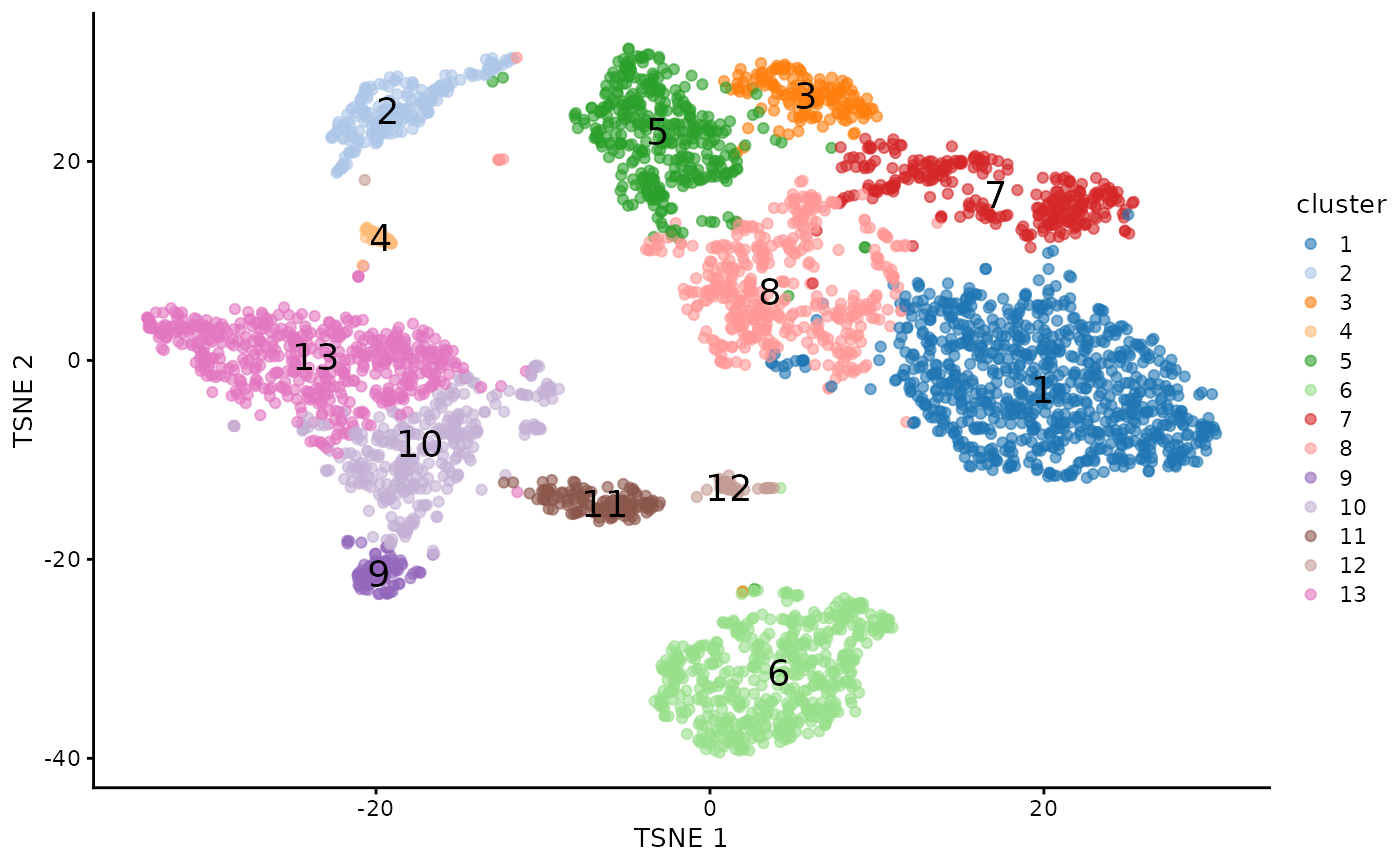
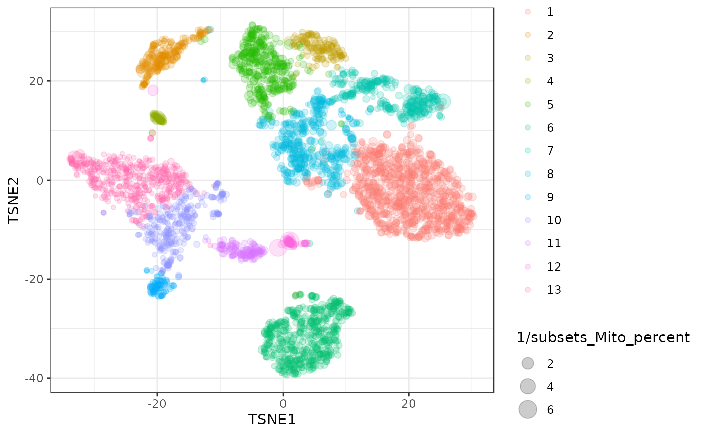
counts_cluster %>%
  ggplot(aes(
    TSNE1, TSNE2,
    color=cluster,
    size = 1/subsets_Mito_percent
  )) +
  geom_point(alpha=0.2) +
  theme_bw()