Side-by-side comparison with standard interfaces

Abstract

Tidybulk is a comprehensive R package for modular transcriptomic data analysis that brings transcriptomics to the tidyverse. It provides a unified interface for data transformation, normalization, filtering, dimensionality reduction, clustering, differential analysis, cellularity analysis, and gene enrichment with seamless integration of SummarizedExperiment objects and tidyverse principles.

tidybulk is a powerful R package designed for modular transcriptomic data analysis that brings transcriptomics to the tidyverse.

Why tidybulk?

Tidybulk provides a unified interface for comprehensive transcriptomic data analysis with seamless integration of SummarizedExperiment objects and tidyverse principles. It streamlines the entire workflow from raw data to biological insights.

Scientific Citation

Mangiola, Stefano, Ramyar Molania, Ruining Dong, Maria A. Doyle, and Anthony T. Papenfuss. 2021. “Tidybulk: An R tidy framework for modular transcriptomic data analysis.” Genome Biology 22 (42). https://doi.org/10.1186/s13059-020-02233-7

Genome Biology - tidybulk: an R tidy framework for modular transcriptomic data analysis

Aggregate duplicated `transcripts`

tidybulk provide the aggregate_duplicates function to aggregate duplicated transcripts (e.g., isoforms, ensembl). For example, we often have to convert ensembl symbols to gene/transcript symbol, but in doing so we have to deal with duplicates. aggregate_duplicates takes a tibble and column names (as symbols; for sample, transcript and count) as arguments and returns a tibble with transcripts with the same name aggregated. All the rest of the columns are appended, and factors and boolean are appended as characters.

TidyTranscriptomics

rowData(airway)$gene_name = rownames(airway)
airway.aggr = airway |> aggregate_duplicates(.transcript = gene_name)

Standard procedure (comparative purpose)

temp = data.frame(
    symbol = dge_list$genes$symbol,
    dge_list$counts
)
dge_list.nr <- by(temp, temp$symbol,
    function(df)
        if(length(df[1,1])>0)
            matrixStats:::colSums(as.matrix(df[,-1]))
)
dge_list.nr <- do.call("rbind", dge_list.nr)
colnames(dge_list.nr) <- colnames(dge_list)

Scale `counts`

We may want to compensate for sequencing depth, scaling the transcript abundance (e.g., with TMM algorithm, Robinson and Oshlack doi.org/10.1186/gb-2010-11-3-r25). scale_abundance takes a tibble, column names (as symbols; for sample, transcript and count) and a method as arguments and returns a tibble with additional columns with scaled data as <NAME OF COUNT COLUMN>_scaled.

TidyTranscriptomics

airway.norm = airway |> identify_abundant(factor_of_interest = dex) |> scale_abundance()

## Warning: The `factor_of_interest` argument of `identify_abundant()` is deprecated as of
## tidybulk 2.0.0.
## ℹ Please use the `formula_design` argument instead.
## ℹ The argument 'factor_of_interest' is deprecated and will be removed in a
##   future release. Please use the 'design' or 'formula_design' argument instead.
## This warning is displayed once every 8 hours.
## Call `lifecycle::last_lifecycle_warnings()` to see where this warning was
## generated.

## tidybulk says: the sample with largest library size SRR1039517 was chosen as reference for scaling

Standard procedure (comparative purpose)

library(edgeR)

dgList <- DGEList(count_m=x,group=group)
keep <- filterByExpr(dgList)
dgList <- dgList[keep,,keep.lib.sizes=FALSE]
# ... additional processing steps ...
dgList <- calcNormFactors(dgList, method="TMM")
norm_counts.table <- cpm(dgList)

We can easily plot the scaled density to check the scaling outcome. On the x axis we have the log scaled counts, on the y axes we have the density, data is grouped by sample and coloured by treatment.

airway.norm |>
    ggplot(aes(counts_scaled + 1, group=.sample, color=`dex`)) +
    geom_density() +
    scale_x_log10() +
    my_theme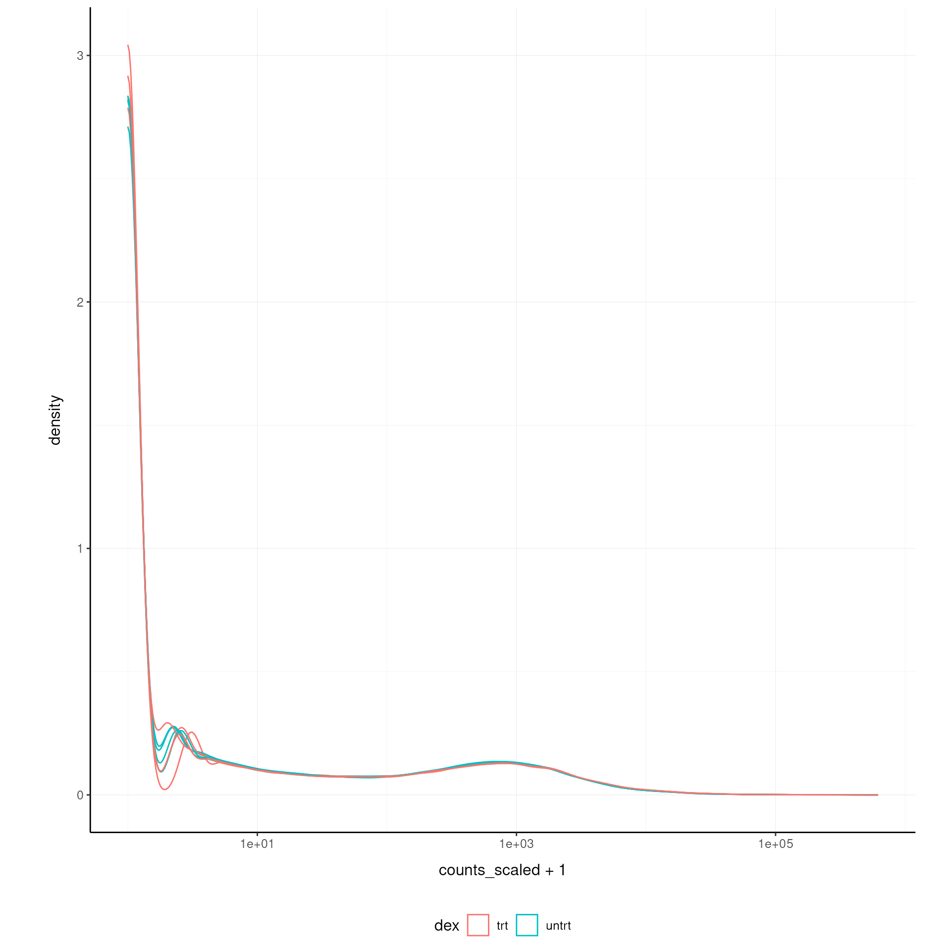

Filter `variable transcripts`

We may want to identify and filter variable transcripts.

TidyTranscriptomics

airway.norm.variable = airway.norm |> keep_variable()

## Getting the 500 most variable genes

Standard procedure (comparative purpose)

library(edgeR)

x = norm_counts.table

s <- rowMeans((x-rowMeans(x))^2)
o <- order(s,decreasing=TRUE)
x <- x[o[1L:top],,drop=FALSE]

norm_counts.table = norm_counts.table[rownames(x)]

norm_counts.table$cell_type = tibble_counts[
    match(
        tibble_counts$sample,
        rownames(norm_counts.table)
    ),
    "cell"
]

Reduce `dimensions`

We may want to reduce the dimensions of our data, for example using PCA or MDS algorithms. reduce_dimensions takes a tibble, column names (as symbols; for sample, transcript and count) and a method (e.g., MDS or PCA) as arguments and returns a tibble with additional columns for the reduced dimensions.

MDS (Robinson et al., 10.1093/bioinformatics/btp616)

TidyTranscriptomics

airway.norm.MDS =
  airway.norm |>
  reduce_dimensions(method="MDS", .dims = 2)

## Getting the 500 most variable genes

## [1] "MDS result_df colnames: sample, 1, 2"

## tidybulk says: to access the raw results do `metadata(.)$tidybulk$MDS`

Standard procedure (comparative purpose)

library(limma)

count_m_log = log(count_m + 1)
cmds = limma::plotMDS(count_m_log, ndim = 3, plot = FALSE)

cmds = cmds %$% 
    cmdscale.out |>
    setNames(sprintf("Dim%s", 1:6))

cmds$cell_type = tibble_counts[
    match(tibble_counts$sample, rownames(cmds)),
    "cell"
]

On the x and y axes axis we have the reduced dimensions 1 to 3, data is coloured by treatment.

airway.norm.MDS |> pivot_sample()  |> select(contains("Dim"), everything())

airway.norm.MDS |>
    pivot_sample() |>
  GGally::ggpairs(columns = 9:11, ggplot2::aes(colour=`dex`))

PCA

TidyTranscriptomics

airway.norm.PCA =
  airway.norm |>
  reduce_dimensions(method="PCA", .dims = 2)

Standard procedure (comparative purpose)

count_m_log = log(count_m + 1)
pc = count_m_log |> prcomp(scale = TRUE)
variance = pc$sdev^2
variance = (variance / sum(variance))[1:6]
pc$cell_type = counts[
    match(counts$sample, rownames(pc)),
    "cell"
]

On the x and y axes axis we have the reduced dimensions 1 to 3, data is coloured by treatment.

airway.norm.PCA |> pivot_sample() |> select(contains("PC"), everything())

airway.norm.PCA |>
     pivot_sample() |>
  GGally::ggpairs(columns = 11:13, ggplot2::aes(colour=`dex`))

Rotate `dimensions`

We may want to rotate the reduced dimensions (or any two numeric columns really) of our data, of a set angle. rotate_dimensions takes a tibble, column names (as symbols; for sample, transcript and count) and an angle as arguments and returns a tibble with additional columns for the rotated dimensions. The rotated dimensions will be added to the original data set as <NAME OF DIMENSION> rotated <ANGLE> by default, or as specified in the input arguments.

TidyTranscriptomics

airway.norm.MDS.rotated =
  airway.norm.MDS |>
    rotate_dimensions(`Dim1`, `Dim2`, rotation_degrees = 45)

Standard procedure (comparative purpose)

rotation = function(m, d) {
    r = d * pi / 180
    ((bind_rows(
        c(`1` = cos(r), `2` = -sin(r)),
        c(`1` = sin(r), `2` = cos(r))
    ) |> as_matrix()) %*% m)
}
mds_r = pca |> rotation(rotation_degrees)
mds_r$cell_type = counts[
    match(counts$sample, rownames(mds_r)),
    "cell"
]

Original On the x and y axes axis we have the first two reduced dimensions, data is coloured by treatment.

airway.norm.MDS.rotated |>
    ggplot(aes(x=`Dim1`, y=`Dim2`, color=`dex` )) +
  geom_point() +
  my_theme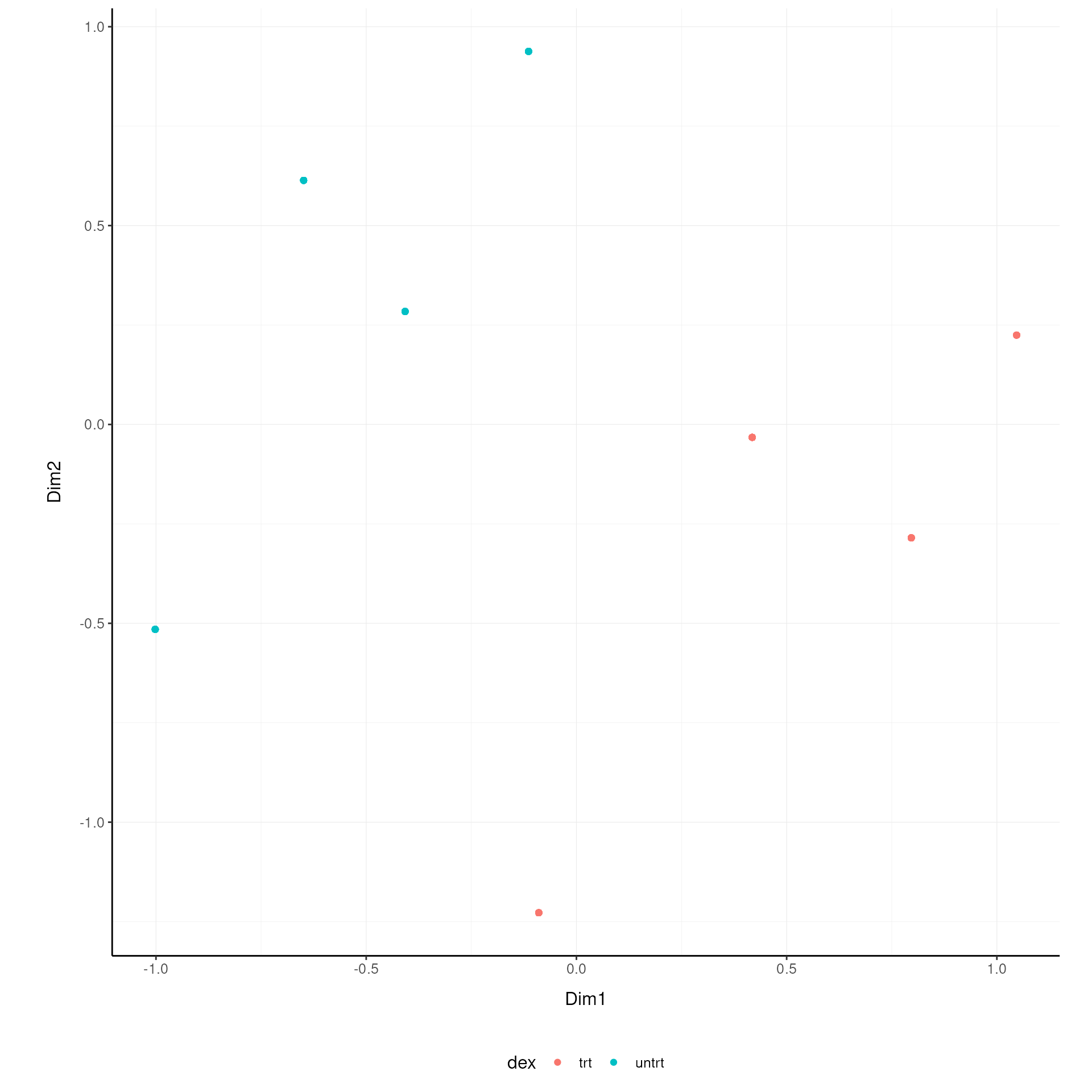

Rotated On the x and y axes axis we have the first two reduced dimensions rotated of 45 degrees, data is coloured by treatment.

airway.norm.MDS.rotated |>
    pivot_sample() |>
    ggplot(aes(x=`Dim1_rotated_45`, y=`Dim2_rotated_45`, color=`dex` )) +
  geom_point() +
  my_theme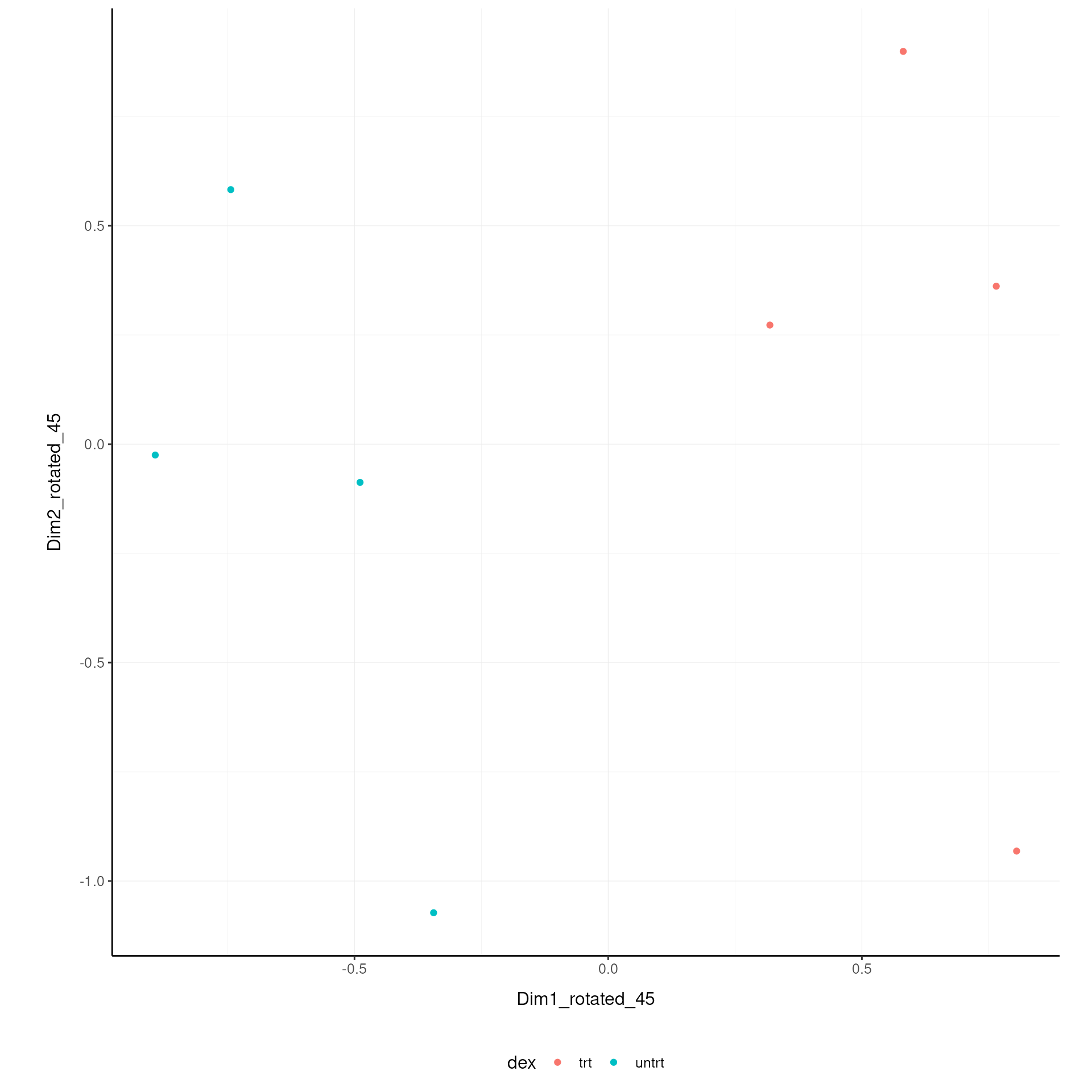

Test `differential abundance`

We may want to test for differential transcription between sample-wise factors of interest (e.g., with edgeR). test_differential_expression takes a tibble, column names (as symbols; for sample, transcript and count) and a formula representing the desired linear model as arguments and returns a tibble with additional columns for the statistics from the hypothesis test (e.g., log fold change, p-value and false discovery rate).

TidyTranscriptomics

airway.de =
    airway |>
    test_differential_expression( ~ dex, method = "edgeR_quasi_likelihood") |>
  pivot_transcript()
airway.de

Standard procedure (comparative purpose)

library(edgeR)

dgList <- DGEList(counts=counts_m,group=group)
keep <- filterByExpr(dgList)
dgList <- dgList[keep,,keep.lib.sizes=FALSE]
dgList <- calcNormFactors(dgList)
design <- model.matrix(~group)
dgList <- estimateDisp(dgList,design)
fit <- glmQLFit(dgList,design)
qlf <- glmQLFTest(fit,coef=2)
topTags(qlf, n=Inf)

The functon test_differential_expression operated with contrasts too. The constrasts hve the name of the design matrix (generally )

airway.de =
    airway |>
    identify_abundant(factor_of_interest = dex) |>
    test_differential_expression(
        ~ 0 + dex,                  
        .contrasts = c( "dexuntrt - dextrt"),
        method = "edgeR_quasi_likelihood"
    ) |> 
  pivot_transcript()

Adjust `counts`

We may want to adjust counts for (known) unwanted variation. adjust_abundance takes as arguments a tibble, column names (as symbols; for sample, transcript and count) and a formula representing the desired linear model where the first covariate is the factor of interest and the second covariate is the unwanted variation, and returns a tibble with additional columns for the adjusted counts as <COUNT COLUMN>_adjusted. At the moment just an unwanted covariates is allowed at a time.

TidyTranscriptomics

airway.norm.adj =
    airway.norm     |> adjust_abundance(    .factor_unwanted = cell, .factor_of_interest = dex, method="combat")

Standard procedure (comparative purpose)

library(sva)

count_m_log = log(count_m + 1)

design =
        model.matrix(
            object = ~ factor_of_interest + batch,
            data = annotation
        )

count_m_log.sva =
    ComBat(
            batch = design[,2],
            mod = design,
            ...
        )

count_m_log.sva = ceiling(exp(count_m_log.sva) -1)
count_m_log.sva$cell_type = counts[
    match(counts$sample, rownames(count_m_log.sva)),
    "cell"
]

Deconvolve `Cell type composition`

We may want to infer the cell type composition of our samples (with the algorithm Cibersort; Newman et al., 10.1038/nmeth.3337). deconvolve_cellularity takes as arguments a tibble, column names (as symbols; for sample, transcript and count) and returns a tibble with additional columns for the adjusted cell type proportions.

Note: Cellularity deconvolution requires gene symbols that match the reference data. The airway dataset uses Ensembl IDs, so this example is commented out.

TidyTranscriptomics

# Requires gene symbols that match reference data
# airway.cibersort =
#   airway |>
#   deconvolve_cellularity( cores=1, prefix = "cibersort__") |> 
#   pivot_sample()

Standard procedure (comparative purpose)

source("CIBERSORT.R")
count_m |> write.table("mixture_file.txt")
results <- CIBERSORT(
    "sig_matrix_file.txt",
    "mixture_file.txt",
    perm=100, QN=TRUE
)
results$cell_type = tibble_counts[
    match(tibble_counts$sample, rownames(results)),
    "cell"
]

Note: The plotting code is commented out as the deconvolution step is not executed.

# airway.cibersort |>
#   pivot_longer(
#       names_to= "Cell_type_inferred", 
#       values_to = "proportion", 
#       names_prefix ="cibersort__", 
#       cols=contains("cibersort__")
#   ) |>
#   ggplot(aes(x=Cell_type_inferred, y=proportion, fill=cell)) +
#   geom_boxplot() +
#   facet_wrap(~cell) +
#   my_theme +
#   theme(axis.text.x = element_text(angle = 90, hjust = 1, vjust = 0.5), aspect.ratio=1/5)

Cluster samples

We may want to cluster our samples based on the transcriptomic profiles. cluster_elements takes as arguments a tibble, column names (as symbols; for sample, transcript and count) and returns a tibble with additional columns for the cluster labels.

TidyTranscriptomics

airway.norm.cluster =
    airway.norm |>
    cluster_elements(method="kmeans", centers = 2)

Standard procedure (comparative purpose)

library(stats)

count_m_log = log(count_m + 1)
count_m_log_centered = count_m_log - rowMeans(count_m_log)

kmeans_result = kmeans(t(count_m_log_centered), centers = 2)

cluster_labels = kmeans_result$cluster

Test differential abundance

We may want to test for differential abundance between conditions. test_differential_abundance takes as arguments a tibble, column names (as symbols; for sample, transcript and count) and a formula representing the desired linear model, and returns a tibble with additional columns for the statistics from the hypothesis test (e.g., log fold change, p-value and false discovery rate).

TidyTranscriptomics

airway.norm.de =
    airway.norm |>
    test_differential_abundance(~ dex, method="edgeR_quasi_likelihood")

## tidybulk says: The design column names are "(Intercept), dexuntrt"

## tidybulk says: to access the DE object do `metadata(.)$tidybulk$edgeR_quasi_likelihood_object`
## tidybulk says: to access the raw results (fitted GLM) do `metadata(.)$tidybulk$edgeR_quasi_likelihood_fit`

Standard procedure (comparative purpose)

library(edgeR)

count_m_log = log(count_m + 1)

design = model.matrix(~ dex, data = annotation)

dge = DGEList(counts = count_m)
dge = calcNormFactors(dge)
dge = estimateDisp(dge, design)

fit = glmQLFit(dge, design)
qlf = glmQLFTest(fit, coef=2)

results = topTags(qlf, n = Inf)

Conclusion

sessionInfo()

## R version 4.5.1 (2025-06-13)
## Platform: x86_64-pc-linux-gnu
## Running under: Ubuntu 24.04.2 LTS
## 
## Matrix products: default
## BLAS:   /usr/lib/x86_64-linux-gnu/openblas-pthread/libblas.so.3 
## LAPACK: /usr/lib/x86_64-linux-gnu/openblas-pthread/libopenblasp-r0.3.26.so;  LAPACK version 3.12.0
## 
## locale:
##  [1] LC_CTYPE=en_US.UTF-8       LC_NUMERIC=C              
##  [3] LC_TIME=en_US.UTF-8        LC_COLLATE=en_US.UTF-8    
##  [5] LC_MONETARY=en_US.UTF-8    LC_MESSAGES=en_US.UTF-8   
##  [7] LC_PAPER=en_US.UTF-8       LC_NAME=C                 
##  [9] LC_ADDRESS=C               LC_TELEPHONE=C            
## [11] LC_MEASUREMENT=en_US.UTF-8 LC_IDENTIFICATION=C       
## 
## time zone: UTC
## tzcode source: system (glibc)
## 
## attached base packages:
## [1] stats4    stats     graphics  grDevices utils     datasets  methods  
## [8] base     
## 
## other attached packages:
##  [1] airway_1.29.0                   tidySummarizedExperiment_1.19.0
##  [3] SummarizedExperiment_1.39.1     Biobase_2.69.0                 
##  [5] GenomicRanges_1.61.1            Seqinfo_0.99.2                 
##  [7] IRanges_2.43.0                  S4Vectors_0.47.0               
##  [9] BiocGenerics_0.55.1             generics_0.1.4                 
## [11] MatrixGenerics_1.21.0           matrixStats_1.5.0              
## [13] tidybulk_1.99.2                 ttservice_0.5.3                
## [15] ggrepel_0.9.6                   ggplot2_3.5.2                  
## [17] magrittr_2.0.3                  tibble_3.3.0                   
## [19] tidyr_1.3.1                     dplyr_1.1.4                    
## [21] knitr_1.50                      BiocStyle_2.37.1               
## 
## loaded via a namespace (and not attached):
##  [1] DBI_1.2.3            rlang_1.1.6          compiler_4.5.1      
##  [4] RSQLite_2.4.2        mgcv_1.9-3           png_0.1-8           
##  [7] systemfonts_1.2.3    vctrs_0.6.5          sva_3.57.0          
## [10] stringr_1.5.1        pkgconfig_2.0.3      crayon_1.5.3        
## [13] fastmap_1.2.0        XVector_0.49.0       ellipsis_0.3.2      
## [16] labeling_0.4.3       utf8_1.2.6           rmarkdown_2.29      
## [19] ragg_1.4.0           purrr_1.1.0          bit_4.6.0           
## [22] xfun_0.53            cachem_1.1.0         jsonlite_2.0.0      
## [25] blob_1.2.4           DelayedArray_0.35.2  BiocParallel_1.43.4 
## [28] parallel_4.5.1       R6_2.6.1             bslib_0.9.0         
## [31] stringi_1.8.7        RColorBrewer_1.1-3   limma_3.65.3        
## [34] genefilter_1.91.0    jquerylib_0.1.4      Rcpp_1.1.0          
## [37] bookdown_0.43        splines_4.5.1        Matrix_1.7-3        
## [40] tidyselect_1.2.1     abind_1.4-8          yaml_2.3.10         
## [43] codetools_0.2-20     lattice_0.22-7       withr_3.0.2         
## [46] KEGGREST_1.49.1      evaluate_1.0.4       desc_1.4.3          
## [49] survival_3.8-3       Biostrings_2.77.2    pillar_1.11.0       
## [52] BiocManager_1.30.26  plotly_4.11.0        scales_1.4.0        
## [55] xtable_1.8-4         glue_1.8.0           lazyeval_0.2.2      
## [58] tools_4.5.1          data.table_1.17.8    annotate_1.87.0     
## [61] locfit_1.5-9.12      fs_1.6.6             XML_3.99-0.18       
## [64] grid_4.5.1           AnnotationDbi_1.71.1 edgeR_4.7.3         
## [67] nlme_3.1-168         cli_3.6.5            textshaping_1.0.1   
## [70] fansi_1.0.6          S4Arrays_1.9.1       viridisLite_0.4.2   
## [73] gtable_0.3.6         sass_0.4.10          digest_0.6.37       
## [76] SparseArray_1.9.1    org.Hs.eg.db_3.21.0  htmlwidgets_1.6.4   
## [79] farver_2.1.2         memoise_2.0.1        htmltools_0.5.8.1   
## [82] pkgdown_2.1.3        lifecycle_1.0.4      httr_1.4.7          
## [85] statmod_1.5.0        bit64_4.6.0-1

Stefano Mangiola

2025-08-21

Why tidybulk?

Scientific Citation

Aggregate duplicated `transcripts`

Scale `counts`

Filter `variable transcripts`

Reduce `dimensions`

Rotate `dimensions`

Test `differential abundance`

Adjust `counts`

Deconvolve `Cell type composition`

Cluster samples

Test differential abundance

Conclusion

Side-by-side comparison with standard interfaces

Stefano Mangiola

2025-08-21

Why tidybulk?

Scientific Citation

Aggregate duplicated transcripts

Scale counts

Filter variable transcripts

Reduce dimensions

Rotate dimensions

Test differential abundance

Adjust counts

Deconvolve Cell type composition

Cluster samples

Test differential abundance

Conclusion

Aggregate duplicated `transcripts`

Scale `counts`

Filter `variable transcripts`

Reduce `dimensions`

Rotate `dimensions`

Test `differential abundance`

Adjust `counts`

Deconvolve `Cell type composition`